
Abstract
Previous studies indicate that both electroencephalogram (EEG) spectral power (in particular the alpha and theta band) and event-related potentials (ERPs) (in particular the P300) can be used as a measure of mental work or memory load. We compare their ability to estimate workload level in a well-controlled task. In addition, we combine both types of measures in a single classification model to examine whether this results in higher classification accuracy than either one alone. Participants watched a sequence of visually presented letters and indicated whether or not the current letter was the same as the one (n instances) before. Workload was varied by varying n. We developed different classification models using ERP features, frequency power features or a combination (fusion). Training and testing of the models simulated an online workload estimation situation. All our ERP, power and fusion models provide classification accuracies between 80% and 90% when distinguishing between the highest and the lowest workload condition after 2 min. For 32 out of 35 participants, classification was significantly higher than chance level after 2.5 s (or one letter) as estimated by the fusion model. Differences between the models are rather small, though the fusion model performs better than the other models when only short data segments are available for estimating workload.
Export citation and abstract BibTeX RIS
Introduction
Brain–computer interfaces (BCIs) traditionally harness consciously generated brain signals to control a device, such as those occurring when mentally imagining different types of movement in order to move a cursor. These types of BCIs (active BCIs; Zander and Kothe 2011) could potentially be very helpful for disabled (paralyzed) individuals by replacing the usual channels of communication and control that healthy individuals use, i.e. hands or mouth. BCIs that make use of spontaneously generated brain signals as an additional channel that provides information about the user's state (passive BCIs; Zander and Kothe 2011) could be useful for healthy individuals in the short term (Coffey et al 2010, Zander and Kothe 2011)4. Such a passive BCI could for example monitor workload online through electroencephalogram (EEG) and issue warnings to request help, or adapt a task if needed. Wilson and Russell (2007) showed that in a simulated uninhabited aerial vehicle task, performance improved when the operator's task was alleviated at times when a combination of psychophysiological measures indicated a high workload, compared to when the same alleviation was provided at random times. While changes in automation level could simply be initiated by the user (e.g. the use of autopilot in aviation), several studies have found that the need to monitor one's own workload further increases workload and leads to reduced performance (Bailey et al 2006). Also, operators may not always be the best judges of when levels of automation need to change. In this study we examine in a controlled experiment to what extent (combining) two different aspects of EEG, spectral power and event-related potential (ERP) measures, contribute to workload estimation with the ultimate purpose to estimate workload online and use these estimates to support the user (as in passive BCIs).
Mental workload is usually defined as the ratio between task demands and a person's capacity (Kantowitz 1988, O'Donnell and Eggemeier 1986) where workload is high when task demands are close to exceeding capacity. Knowing an individual's workload would be useful in monitoring and assisting people at work, as well as in evaluating and designing systems or working conditions. Performance measures like work pace and accuracy can be useful indicators of workload in some cases, but usually it is undesirable to wait until performance is overtly decreased. In addition, work pace and accuracy are often difficult to determine (Collet et al 2009, Veltman and Gaillard 1996). Another way to measure workload is through subjective rating scales like the NASA-TLX, SWAT (discussed in Nygren 1991) and RSME (Zijlstra 1993). However, repeatedly gauging workload in such a way is distracting and burdens the worker with an extra task. Delaying workload assessment in order to avoid this intrusion may introduce effects of memory lapses and operator bias (Moroney et al 1995). Moreover, rating scales can be intentionally or unintentionally distorted. An example of this is a study by Vogt et al (2002) where air traffic controllers' workload reports were dominated by the amount of traffic while it was clear from other variables that this was only one of the relevant factors. Physiological indicators could provide a continuous measurement of workload that does not distract the operator with questions and is independent of both overt performance measures and possibly distorted retrospective reports (Wilson and Eggemeier 1991).
Studies on physiological correlates of workload (or mental load) go back to at least the early 1960s (Kalsbeek and Ettema 1963). A range of variables has been examined over the years such as heart rate, different types of heart rate variability, pupil size, eye blink frequency and duration, saccade and fixation related measures, electrodermal measures, respiration, blood pressure, chemical measures, EMG and neurophysiological variables derived from EEG. To our knowledge, a substantial, recent review of physiological responses to workload is lacking. There does not seem to be an obvious 'winning' variable that can effectively be used to determine workload. One review study (Hancock 1985) suggested heart rate variability as the most reliable measure, whereas another (Vogt et al 2006) reviewed 19 studies in which heart rate variability was not even recorded. In these studies, heart rate seemed to be relatively reliable. Studies that examined EEG spectral variables next to other physiological variables such as different eye and heart related measures, concluded or suggested EEG to be the most sensitive or promising indicator of workload (Berka et al 2007, Brookings et al 1996, Taylor et al 2010, Christensen et al 2012). In the present study, we recorded a range of physiological variables simultaneously but for the current manuscript we focus on EEG.
Several studies reported a correlation between work or memory load and power in certain EEG frequency bands—in particular alpha (8–12 Hz) and theta (4–8 Hz). Alpha has been linked to idling (Pfurtscheller et al 1996), default mode brain activity (Jann et al 2009, Laufs et al 2003) and cortical inhibition (van Dijk et al 2008, Foxe et al 1998, Brouwer et al 2009). This would all roughly be consistent with alpha power varying with different levels of workload. More explicitly, alpha has been suggested to indicate mental effort since a decrease in alpha power is associated with an increase in arousal, resource allocation or workload (e.g. Ray and Cole 1985, Fink et al 2005, Pfurtscheller et al 1996, Sterman et al 1994). While the exact location of the effect varies with modality and task (Pfurtscheller et al 1994) for effortful and attentive processing alpha reduction is observed at parietal regions (Klimesch et al 2000, Keil et al 2006). Evidence for an association between theta and working memory processes or mental effort has been summarized in several reviews by Klimesch (1996, 1997, 1999). Theta increases as task requirements increase (e.g. Miyata et al 1990, Jensen and Tesche 2002, Esposito et al 2009, Raghavachari et al 2001). This theta increase is most profound over frontal electrode locations. A number of studies on workload reported both alpha and theta effects (e.g. Brookings et al 1996, Gevins et al 1998, Fournier et al 1999, Gundel and Wilson 1992). Besides alpha and theta, power in some other frequency bands has been reported to respond to varying workload (beta and delta: Brookings et al 1996, gamma: Laine et al 2002).
Besides EEG spectral variables, ERPs potentially convey relevant information about an individual's workload. The P300 reflects attentional and working memory processes (Polich and Kok 1995, Polich 2007). The classic paradigm to elicit a P300 is the oddball paradigm (Polich and Kok 1995). Observers are presented with a series of two types of stimuli where one of them (the oddball) occurs infrequently. Observers are usually asked to pay attention to the oddball, for instance by counting the number of times that it is presented. The P300 associated with the oddball or target is higher than the one associated with the non-target. In order to elicit a P300, targets need not physically stand out from the non-targets—voluntary attention to one target stimulus embedded in several similar non-target stimuli is also sufficient. This fact is gratefully used in BCIs such as the P300 speller (Farwell and Donchin 1988). Even though the exact underlying mechanism is under debate (Kok 2001) numerous studies found that the P300 decreases with increasing memory or workload (Evans et al 2011, Pratt et al 2011, Watter et al 2001, Allison and Polich 2008, Kida et al 2004, Raabe et al 2005). This effect was found even though these studies differ with respect to whether the eliciting stimuli were an integral part of the task or whether they were presented simultaneously with another, main task that was varied in difficulty. The reported studies also differed in including only the target or also the non-target stimuli when determining the P300 amplitude. Allison and Polich (2008) did not even present non-target stimuli, but presented participants only with target stimuli at irregular intervals and found lower P300 amplitudes when participants were playing a high compared to a low workload level of a computer game. Besides the P300, earlier ERP components like the N100 (Kramer et al 1995, Ullsperger et al 2001, Allison and Polich 2008), the N200 (Kramer et al 1995), the P1 (Pratt et al 2011) and a positive–negative component between 140 and 280 ms (Missonnier et al 2003 2004) have been found to respond to task difficulty or workload. Finally, late positive or negative slow waves have been related to high memory load (Ruchkin et al 1990) and amount of resource allocation (Rösler et al 1997).
As far as we know, the effect of varying workload on the power in different EEG frequency bands and on ERP related measures has never been examined within one study as was also noted in a recent review (van Erp et al 2010). We will do that here in order to get an impression of their relative ability to estimate an individual's workload level. In addition, we will examine whether combining these two types of measures improves this estimation considering that spectral power and ERPs differ with respect to their evolution over time and could carry complementary information about the level of workload. An indication of complementary value of spectral power and ERPs is given by Missonnier et al (2007) who found that using both spectral and ERP components as measured during a demanding 2-back workload task contributed to predicting decline in mild cognitive impairment compared to either one alone.
We used the n-back task to manipulate workload, or more specifically memory load (Kirchner 1958). Memory load is considered to be a major component and reasonable approximation of workload (Berka et al 2007, Grimes et al 2008). The elegant properties of the n-back task have led to its extensive, wide-spread use such as a tool to manipulate workload in neuroimaging (for a meta-analysis of brain regions involved in working memory see Owen et al (2005)) and as a tool to measure cognitive performance under various conditions (e.g. Moore et al 2009). In the n-back task participants view successively presented letters. For each letter they have to decide whether or not it is the same as the one presented n letters before. By increasing 'n' memory load can be increased without affecting visual input and frequency and type of motor output. These factors can act as confounding variables that impede the interpretation of results of previous studies on correlates of workload (e.g. Collet et al 2009, Vogt et al 2006, Veltman and Gaillard 1998, Wilson and Russell 2003, 2007, Christensen et al 2012). Another advantage of the n-back task for this particular study is that it involves stimuli that we can use to study ERPs so that adding secondary stimuli for this purpose is not needed.
We are interested in estimating the level of workload in real time to allow these estimates to be used for online support. This requires us to judge from a short fragment of data of a particular individual whether the workload level is low or high. Classic ERP and EEG spectral analyses that examine general differences between conditions based on large amounts of data segments and multiple participants are not particularly suitable for this. A suitable method for sorting few a short fragments of physiological data of one individual into different categories is classification analysis. This type of analysis is commonly used in BCIs (van Gerven et al 2009a, Blankertz et al 2004, Müller et al 2004, Lotte et al 2007). In short, features that are expected to carry information of interest are determined, e.g. power at certain frequency bands or the voltage in a certain time window after stimulus presentation. Then a classification algorithm (such as a support vector machine; SVM) is fed with feature vectors, i.e. the values of data fragments, and the labels as to which class these feature vectors belong to. Thus, in this phase one needs to know the class of the fragments. Based on the known classes, the most informative data characteristics are determined and the model is trained. The resulting trained model is subsequently used to classify new, unseen data in (hopefully) appropriate classes. The main dependent variable in our manuscript is classification accuracy: the accuracy with which a model, tuned to labeled training data of an individual, can classify new data with respect to the different workload levels of the task. As just described, EEG classification is usually done with individually trained models. Particularly for classifying workload, there are indications that the individual adjustment of the classifier is of importance. Based on their own data and data of others (Jensen et al 2002, Prinzel et al 2001), Grimes et al (2008) pointed out that memory load affects EEG quite differently between individuals, though when averaged over large numbers of participants data usually exhibit trends as reported in the literature. It is not so surprising that EEG responses to varying workload are different between individuals while being relatively consistent within individuals when considering the different physical properties of individuals' cortices, different competencies, different strategies and different mental states like arousal and motivation that can all vary with workload level.
Over participants, we specifically expect power in the alpha frequency to decrease, theta to increase and the P300 amplitude to decrease with workload level. Consistent with the P300 amplitude being higher for a target than a non-target in an oddball paradigm, P300 workload studies that used an n-back task report the amplitude to be higher for (less frequently presented) targets than for (more frequently presented) non-targets (Wild-Wall et al 2011, Evans et al 2011, Watter et al 2001—where the first two studies only included correct responses and the last one did not). We hypothesize that since distinguishing between a target and non-target will become more difficult with increasing workload level, the difference between target and non-target P300 amplitude will decrease with workload level. The features of our spectral power and ERP classification models will be chosen in accordance with these expectations and classification accuracies compared. We expect classification models combining spectral power and ERP related features to perform best. Training and testing of classification models will simulate an online workload estimation situation.
Methods
Participants
Thirty-five participants took part in the experiment. They were recruited through the TNO participant pool or acquainted with one of the authors. Participants were aged between 19 and 40 years (mean age 27) and 16 of the participants were male. One participant was left-handed. The experiment was performed in accordance with the local ethics guidelines and participants gave written informed consent.
Materials
Stimuli (letters), rating scale mental effort (RSME) workload scales and announcements about the type of the n-back task to follow were presented on a Tobii T60 Eye Tracker monitor, at a distance of about 50 cm from the participants' eyes. Feedback about task performance was presented through Labtec LCS-1050 speakers in the form of beeps. Participants used a keyboard to indicate whether presented letters were targets or non-targets. Which of the keys (1 or 2 on the numerical pad) indicated 'target' and which 'non-target' was counterbalanced between participants. Participants used the mouse to rate subjective workload on a scale (RSME) when asked.
EEG was recorded through a g.tec USBamp and g.tec Au electrodes placed at Pz, FCz, Fz, C3, C4, F3 and F4, referenced to linked mastoid electrodes. A ground electrode was placed at FPz. To measure EOG (electrooculogram) we used g.tec Au disk electrodes or self-adhesive electrodes alternatively (Kendall Neonatal Ag/AgCl ECG electrodes): two were attached at the outer canthi of the left and right eye; two additional ones were attached above and below the right eye. The left and right EOG electrodes as well as the upper and lower EOG electrodes were referenced to each other. The impedance of all EEG and EOG electrodes was kept below 5 kΩ.
We used the RSME scale (Zijlstra 1993) to measure subjectively experienced mental effort. This scale runs from 0 to 150 with higher values reflecting higher workload. It has nine descriptors along the axis, e.g. 'not effortful' at value 2 and 'rather effortful' at value 58. Verwey and Veltman (1996) concluded this simple one-dimensional scale to be more sensitive than the often-used NASA-TLX (Hart and Staveland 1988).
We recorded several measures that are not further analyzed in the current manuscript: pupil size (using an eye tracker integrated with the lower part of the monitor), ECG (self-adhesive electrodes just below the right collarbone, just below the left lower rib and above the right hip), skin conductance (two self-adhesive electrodes on the palm of the left hand that was not used for pressing the keys) and respiration (an elastic band around the waist at the height of the lower side of the sternum). A video recording of the participant's face was made and participants filled out a personality questionnaire (The Big Five Inventory). All physiological signals were synchronized using the TCAP signal from The Observer XT (Zimmerman et al 2009).
Task
Participants viewed letters, successively presented on a screen. For each letter, they pressed a button to indicate whether the letter was a target or a non-target. In the 0-back condition, the letter x is the target. In the 1-back condition, a letter is a target when it is the same as the one before. In the 2-back condition, a letter is a target when it is the same as two letters before. With this version of the n-back task, the level of workload is varied without varying visual input or frequency and type of motor output (button presses). A 3-back condition was not used, due to evidence that many participants find it too difficult and tend to give up (Izzetoglu et al 2007, Ayaz et al 2007).
Participants were informed after every button press whether it was a correct decision by a high (correct) or a low (incorrect) pitched tone. This was to help the participant, who in our experiment switched rather often between n-back conditions, and to increase motivation since the participant knew the experiment leader would hear the sounds as well.
Stimuli
The letters used in the n-back task were black (font style: Matlab standard, approximately 3 cm high) and were presented on a light gray background. The letters were presented for 500 ms followed by a 2000 ms inter-stimulus interval during which the letter was replaced by a fixation cross. In all conditions, 33% of letters were targets. Except for the letter x in the 0-back task, letters were randomly selected from English consonants. Vowels were excluded to reduce the likeliness of participants developing chunking strategies which reduce mental effort, as suggested in Grimes et al (2008).
Design
The three conditions (0-back, 1-back, 2-back) were presented in 2 min blocks divided across four sessions. Each session consisted of two repetitions of each of the three blocks. Thus, for each of the three conditions participants performed 4 sessions * 2 repetitions = 8 blocks. In each block, 48 letters were presented, 16 of which were targets. The blocks were presented in pseudorandom order, such that each condition was presented once in the first half of the session and once in the second half of the session, and that blocks of the same condition never occurred directly after each other. Before each session was a baseline block of 2 min in which the participant quietly fixated a cross on the screen.
Procedure
Upon entering the lab, participants were explained about the experimental procedure. They then read and signed an informed consent form, and filled out the Big Five Inventory. The physiological sensors were attached and participants practiced the task. All three conditions were practiced until the participant and experimental leader were convinced that the task was clear. Regardless of this, all participants completed at least one block of the 2-back task. It was stressed that the 2-back task could be difficult for the participants, but that they should keep trying to do as well as possible. Participants were asked to avoid movement as much as possible while performing the task and to use the breaks in between the blocks to make necessary movements. Before the start of each block, the participant was informed about the nature of the block (rest, 0-back, 1-back or 2-back) via the monitor. After each block, the RSME scale was presented and the participant rated subjective mental effort by clicking the appropriate location on the scale using the mouse. The next block started after the participant indicated his/her readiness by pressing a button. Between sessions, participants had longer breaks—chatting with the experiment leader or having a drink.
Analysis
EEG and EOG data were filtered by a 0.1 Hz high pass and a 100 Hz low pass filter and sampled with a frequency of 256 Hz (USB Biosignal Amplifier, g.tecmedical engineering GmbH). Afterward data were processed and analyzed using Matlab and the FieldTrip open source Matlab toolbox (Oostenveld et al 2011). The classifier that we used was a SVM, as implemented in FieldTrip. Epochs starting at 500 ms before stimulus onset and ending 2000 ms after were shifted such that the mean of the first 500 ms was zero. No eye blink or other artifacts were removed before classification which makes the implementation of online classification easier.
Based on the literature and our own experience we designed five standard classification models with features that reflect ERPs (where ERPs were either synchronized to letters in general or separately to targets and non-targets), power in frequency bands, or both.
- (i)The ERP model used features based on the channel outputs between 0 and 1000 ms after stimulus onset. The signals were resampled to 100 Hz to reduce the amount of features. The ERP model used 7 EEG channels * 101 samples = 707 features.
- (ii)The power model used spectral power features that were estimated using Fourier analysis in a window from –500 to 1500 ms relative to stimulus onset, with frequency bands centered around 2 up to 20 Hz in 0.5 Hz steps (37 in total). The power model used 7 EEG channels * 37 samples = 259 features.
- (iii)The fusion model used all of the features of the ERP and power model, i.e. 707 + 259 = 966 features.
- (iv)The ERP-split model: since we are interested in the potential added value of distinguishing between target and non-target stimuli, we designed another ERP model that is the same as the previous one, except that the features were determined for target and non-target epochs separately. The ERP-split model thus used twice as many features as the ERP model (1414 features).
- (v)The fusion-split model used all of the features of the ERP-split and power model, i.e. 1414 + 259 = 1673 features.
The features were standardized to have mean 0 and standard deviation 1 on the basis of data from the training set.
The first three sessions, each containing two blocks of each n-back condition, were used to train the model parameters to individual participants. The last session was used to evaluate the model's classification accuracy. This simulates estimating workload online, using model parameters that are adjusted to the individual participant in a training phase. As a default, the classification models were trained and applied to distinguish between 0- and 2-back blocks, each containing 2 min of data or 48 trials (letters).
Average classification accuracy (proportion correct in the last session) over all participants was used as the main measure of model performance. Besides classification accuracy, we calculated bitrate (as described in Serby et al (2005)) as a measure of performance that represents the amount of information being communicated, taking into account the number of possible options, the classification accuracy and the time required to communicate the chosen option.
In addition to comparing classification accuracy of the models at the default settings, we examined how classification accuracy depends on the duration of the interval after which a decision is made (i.e. number of trials), we determined classification performance when the models classify conditions that are more similar than 0- and 2-back, we varied the frequency bands and ERP time window to identify the distinguishing information, and we tested whether adding or relying on EOG changes the classification performance.
Since classification accuracy per participant could only take values of 0, 0.25, 0.50, 0.75 and 1 (correct classification of 0 to 4 blocks in the last session), we used Friedman's test rather than repeated measures ANOVAs to evaluate effects of different variables on classification accuracy. This test is less powerful but does not assume a normal distribution or equal variances. Pairwise comparison tests were used to determine whether two accuracies were significantly different from each other, or whether classification accuracy was significantly higher than chance, based on the assumption of an underlying binomial distribution for the accuracy. The effect of n-back condition on behavioral data was evaluated using repeated measures ANOVAs and Tukey post-hoc tests.
Results
Behavioral data
Accuracy and response time
The button press responses to the stimuli could be divided into five categories. In one category no response was given. This only happened in 2% of the trials. In the case a response was given, this could be categorized as either a 'hit' or a 'miss' (when a target was presented) or a 'false alarm' or a 'correct rejection' (when a non-target was presented). To represent the behavioral performance in a single number, we defined the 'fraction correct' as the total number of hits and correct rejections divided by the total number of stimuli. Fraction correct decreased with memory load with averages of 0.96, 0.93 and 0.89 for the 0-back, 1-back and 2-back conditions, respectively (repeated measures ANOVA: F(2,68) = 66.35, p < 0.01). Tukey post-hoc tests show that all three levels are significantly different from each other. The degradation in performance with increasing n-back condition was due to a decrease in hit rate (0.95, 0.88, 0.83 for the 0-back, 1-back and 2-back conditions, respectively5, F(2,68) = 31.48, p < 0.01) and a (small) increase in false alarm rate (0.008, 0.014, 0.0426, F(2,68) = 48.05, p < 0.01) with increasing memory load. Chance performance in this case is a fraction of 0.5 correct if the participant pressed target and non-target buttons randomly, and is 0.66 correct if a participant noticed or guessed that non-targets are more prevalent and always give a 'non-target' response. Only one participant's performance did not deviate significantly from 0.66 in the 2-back condition (0.71) as determined by using a t-test with variance derived from the 'fraction correct' assuming a binomial distribution. All other scores were 0.82 or higher and significantly different from 0.66, indicating that almost all participants were able to perform the task.
A repeated measures ANOVA showed that button press response time increased with memory load with averages of 533, 595 and 698 ms for the 0-back, 1-back and 2-back conditions, respectively (F(2,68) = 56.84, p < 0.01; post-hoc tests showed that all levels significantly differed from each other). There was no effect of stimulus type (target versus non-target) and no interaction between memory load and stimulus type.
Subjective rating: RSME
Perceived mental effort as measured by RSME increased with memory load as expected, with average scores of 35, 43 and 58 for the 0-back, 1-back and 2-back conditions respectively (repeated measures ANOVA F(2,68) = 41.53, p < 0.01; post-hoc tests showed that all levels significantly differed from each other).
Electrophysiological data: general impression
EEG spectral power
Figure 1 indicates the number of participants that show a significant difference in spectral power between the 0-back and 2-back task for different channels and frequency bands. Spectral power was computed over intervals from 500 ms before stimulus onset until 1500 ms after onset. As hypothesized, EEG power that distinguishes between 0-back and 2-back conditions is present in the alpha band (8–12 Hz), especially at Pz. An effect in frontal theta (4–8 Hz) seems to be present, but is less clear.
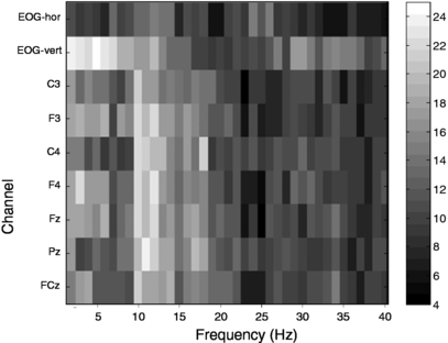
Figure 1. The number of participants (indicated by gray level) that show a significant difference in spectral power between the 0-back and 2-back task for different channels and frequency bands.
Download figure:
Standard imageFigure 2 shows the grand average normalized power spectra (normalized per participant with respect to the average integral over the spectral curves of 0-, 1- and 2-back) for each condition at each of the three midline locations. At Pz, alpha power decreases with memory load. As also indicated by figure 1, other overall effects, such as a reversed effect of workload on theta, are not clear. As found in previous studies (Grimes et al 2008, Jensen et al 2002, Prinzel et al 2001), we observed that the dependence of power spectra on workload varies greatly between participants, with a few participants who show theta peaks that differentiate between conditions as expected.
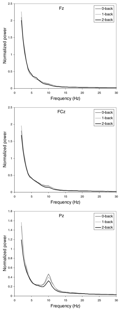
Figure 2. The grand average normalized power spectra for each condition at the midline locations Fz, FCz and Pz.
Download figure:
Standard imageERPs
Figure 3 indicates the number of participants that show a significant voltage difference between the 0-back and 2-back task over channels and time. For this graph the data were filtered using a low-pass filter of 20 Hz and resampled using a sample rate of 20 Hz. ERPs start to differ about 400 ms after stimulus onset with a peak around 700 ms.

Figure 3. The number of participants (indicated by gray level) that show a significant difference in voltage between the 0-back and 2-back task for different channels and time.
Download figure:
Standard imageFigure 4 shows for each midline location and each condition the grand average ERP (left) and the grand average target- and non-target difference trace (right). For these graphs, data were filtered using a low-pass filter of 20 Hz. At Pz, the average target P300 amplitude in the 2-back condition is lower than the 0-back condition as predicted, but the 1-back condition is not in between. Grand average ERPs and difference traces of the data as they entered the classification analysis (i.e. without artifact rejection) seem noisy and do not clearly display the expected patterns. Individual participants show considerable variation in the P300 peak latency at Pz and the presence or absence of multiple peaks. Plots of individual participants suggest that late peaks are largely due to vertical EOG.
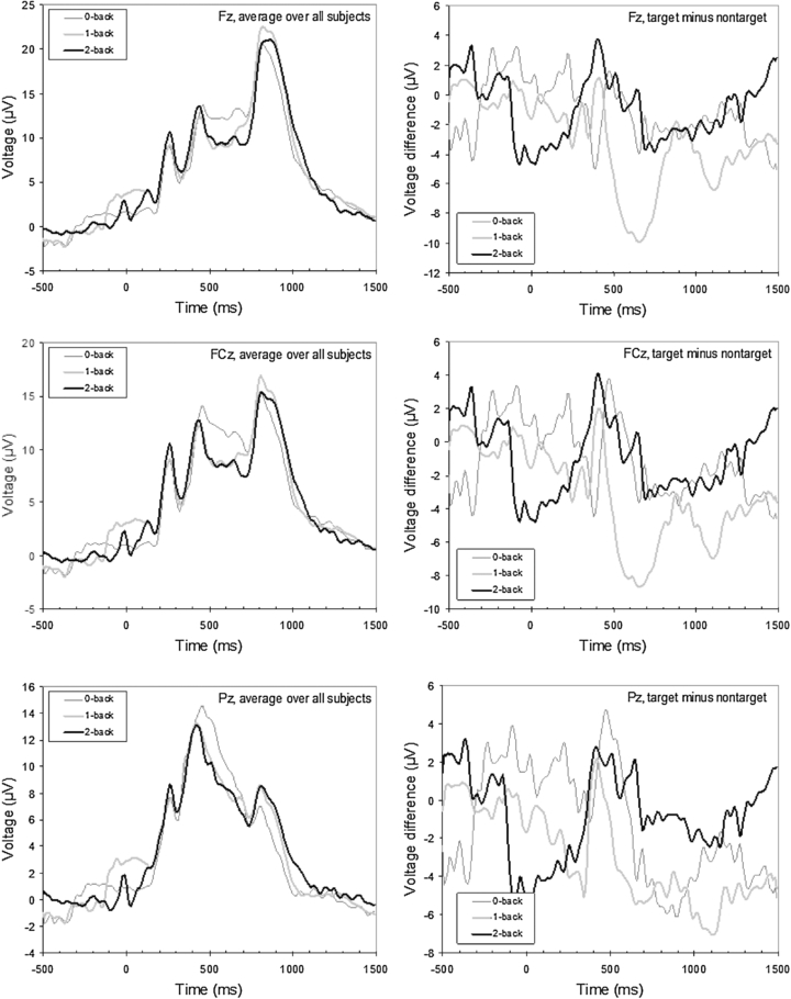
Figure 4. The grand average ERPs at the midline locations Fz, FCz and Pz for each condition (left) and target−non-target difference traces for each midline location and condition (right).
Download figure:
Standard imageElectrophysiological data: classification
General performance and decision time interval
Figure 5(a) shows classification accuracy of the five standard models as a function of the duration of the time interval after which a decision is made as to whether the data fragment is drawn from the 0-back condition or the 2-back condition. The smallest possible unit is one trial (one letter), corresponding to 2.5 s. Note that when the decision is based on a single trial it is impossible to use a model that uses separate features for target and non-target trials. Therefore, for the split models we only derived classification accuracy for the entire block. For all models, average classification performance is significantly above chance (represented by the lower curve in figure 5(a) at all interval durations (p < 0.01). As expected, classification accuracy increases with the duration of the time interval on which the decision is based, or equivalently, the number of stimuli that is used for the classification (Friedman's test: p < 0.01, χ2 = 147.08, df = 6). Friedman's test also reveals a significant effect of model on classification accuracy (p < 0.01, χ2 = 9.85, df = 2), with overall, the fusion model performing best. Pairwise comparison tests show that at short intervals the fusion model is significantly better than the ERP model (interval durations up to 15 s) and the power model (interval durations up to 30 s). On block level (120 s), pairwise comparisons do not reveal any significant differences between any of the five models though the ERP-split model tends to perform best with an average classification accuracy of 0.88. While classification accuracy increases with duration, figure 5(b) shows that the bitrate decreases with duration.
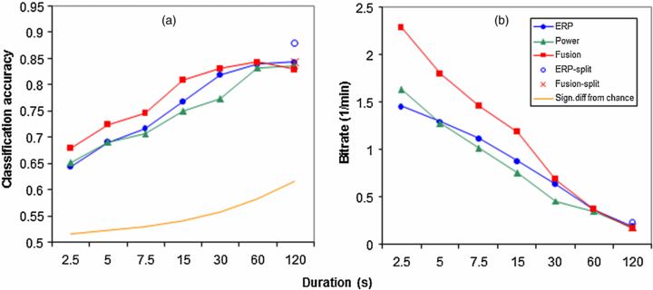
Figure 5. Classification accuracy (a) and bitrate (b) of the five standard models as a function of the time interval after which a decision is made as to whether the data sample is drawn from the 0-back condition or the 2-back condition. Note that the distances between the labels on the x-axis do not represent equidistant time intervals.
Download figure:
Standard imageIn order to get an impression of the variation in classification performance between participants, figure 6 shows the histogram of individual classification accuracy scores for single trials of the fusion model. The model performs (often well) above chance level for 32 out of 35 participants. For both the ERP and the power model, 29 participants perform above chance. Note that using longer time windows for classification increases classification accuracy relative to the single trial performance described here.
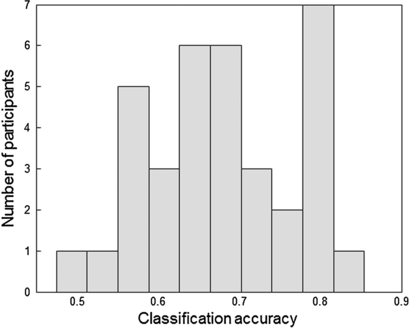
Figure 6. Individual classification accuracy scores for single trials (interval duration of 2.5 s) of the fusion model.
Download figure:
Standard imageClassification of other memory load conditions
Figure 7 shows how well the models perform when they are trained and tested on differentiating the 0- versus the 2-back condition, the 1- versus the 2-back condition and the 0- versus the 1-back condition. All memory load conditions can be distinguished from each other above chance by all models (p < 0.05). As expected, classification accuracy depends on the specific conditions being compared (Friedman's test: main effect of n-back comparison: p < 0.01, χ2 = 57.3, df = 2) with best performance being reached when conditions are classified that are maximally different (0- versus 2-back). Consistent with the data on button press accuracy, response time and RSME that all show a smaller difference between the 0- and 1-back conditions than between the 1- and 2-back conditions, overall classification accuracy is lowest when distinguishing between 0- and 1-back conditions. A Friedman's test did not indicate a significant main effect of model.
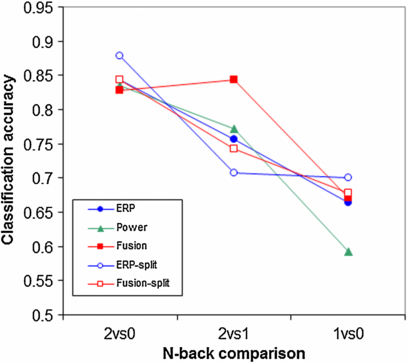
Figure 7. Classification accuracies of the models when they are trained and tested on differentiating the 0- versus the 2-back condition, the 1- versus the 2-back condition and the 0- versus the 1-back condition.
Download figure:
Standard imageVarying features: ERP time window and frequency bands
Figure 8(a) shows the effect of varying the time window of the ERP data that are used. In order to examine whether focusing on the P300 would change performance, we decreased the window from our default window of 0–1000 ms to windows of 200–900 ms and 300–800 ms. Focusing on the P300 did not change performance, i.e. only the accuracy of the ERP-split model seems to decrease when the narrowest window is used, but Friedman's test and pairwise comparisons did not indicate any significant effect of time window. This suggests that most of the information as used by the models is present in the time range between 300 and 800 ms. Time windows of 0–300 and 1500–2000 ms were tested in order to check whether there is any information in the early or late ERP components. While classification accuracy was significantly lower for both ERP models using these early and late windows compared to using medium windows, classification was still above chance. This indicates that there is some, be it little, information to distinguish workload in the first 300 ms after stimulus presentation, as well as after 1500 ms.
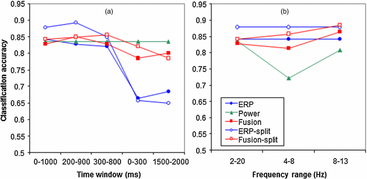
Figure 8. Classification accuracy as a function of time window of the ERP data that are used (a) and as a function of the included frequency bands (b). Note that varying the time window of the ERP does not affect the power model which means that its classification accuracy does not change in (a). Similarly, varying the included frequency bands does not affect the ERP based models and hence, their accuracies remain the same (b).
Download figure:
Standard imageFigure 8(b) examines the relative contribution to classification accuracy of different frequency ranges: our default of 2–20 Hz, theta only (4–8 Hz) and alpha only (8–13 Hz). Friedman's test did not reveal a significant effect of frequency range on the pooled data, but pairwise comparison tests indicated that when the power model only relied on the theta range, it performed significantly worse than when it relied on the broad default range or alpha only.
EOG
The data presented in figures 1 and 3 show that not only EEG but also the EOG channels contain information to distinguish between data from 0- and 2-back conditions. Figure 9 presents classification accuracy for the models based on EEG, both EEG and EOG, and EOG alone. Friedman's test reveals a main effect of the channel types that are being used (p < 0.01, χ2 = 32.2, df = 2) but no significant main effect of model. EEG alone works best while adding or relying on EOG degrades performance. Note that since EOG was not corrected in the EEG data, the EEG and EOG classifications are not completely independent of each other.
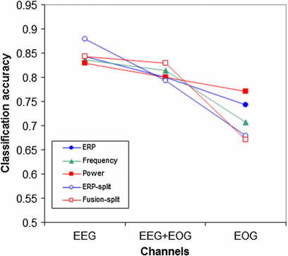
Figure 9. Classification accuracy for the models based on EEG, both EEG and EOG, and EOG alone.
Download figure:
Standard imageAuditory oddball
One potential concern is that our classification results could be (partly) based on auditory oddball stimuli. The number of errors increases with workload and erroneous button presses were followed by low rather than high pitched sounds. To check for the potential influence of the different number of low pitched sounds, we repeated our analyses on single 2.5 s trials from the 0- and 2-back condition, this time including only correct trials associated with high pitch sounds. If the auditory oddball strongly contributed to the classification, the classification of these trials should be worse than that of an equal number of randomly selected trials. This appeared not to be the case (classification accuracies for the power model—high pitch only: 0.64, random selection: 0.65; for the ERP model—high pitch only: 0.66, random selection: 0.65).
Discussion
We examined the separate and combined use of EEG spectral power and ERPs to infer the level of workload that an individual was exposed to in a well-controlled n-back task. Behavioral measures confirm that differences in workload are indeed experienced: with an increase in n-back level, subjective workload increases and task performance decreases. Online determination of workload was simulated and evaluated. Using SVMs that were trained on labeled data of the first three quarters of the experiment we were able to reliably distinguish between different levels of workload in the last quarter of the experiment for 32 out of 35 participants on single trial level (2.5 s) using the fusion model. Classification accuracy of the fusion model was significantly higher than classification accuracy of the power and ERP models when classification decisions were based on few data (up to 6 trials or 15 s for the ERP model and up to 12 trials or 30 s for the power model). There was little difference between classification accuracies of the power and ERP models. Highest classification accuracy scores tended to be reached by the ERP model with features that included information about the identity of the eliciting stimulus (target or non-target)—88% when distinguishing between 0- and 2-back after 48 trials or 120 s. Overall, we conclude that when workload estimates can be made on the basis of relatively long data fragments (therewith improving accuracy), either ERP or power features can be used, but a combination of features performs especially well when few data are available to base the decision on.
Power in the alpha and less so in the theta band generally seemed to contain the most relevant features for distinguishing the highest and lowest n-back level in the models based on spectral power (figures 1, 2 and 8(b)). However, a large individual spread in patterns of spectral power responses stressed the importance of individually tuned classification models. Grand average ERPs and difference traces (figure 4) did not clearly confirm our expectations of a decreasing P300 with increasing workload and of a smaller difference between non-target and target ERPs in high compared to low n-back conditions. Note that differences between participants can obscure effects in grand averages, while individual differences are taken into account in the individually trained classification models. Indeed, results from classification analyses dealing with the same data indicated that the bulk of the information was present in a time interval consistent with the P300. In addition, classification accuracy tended to be higher when the distinction between target and non-target ERPs was preserved in the features. Some effect of early and late ERP components was indicated by better than chance classification between the highest and lowest n-back level when intervals up to 300 ms after stimulus onset were used, as well as intervals between 1500 and 2000 ms. Our results also showed that EOG contained useful information for classification. Further analysis (in which we also aim to include other data about the eyes as provided by the Tobii eye tracker such as pupil size) may clarify what this information is and how we can best make use of it in a practical workload monitoring system.
Combining spectral power and ERP features in the fusion models resulted in improved classification accuracy, especially when classification was based on few data. This is not simply because 'the more features, the better', as shown by cases where classification accuracy tended to decrease after adding extra features (e.g. when adding power features to the ERP-split model, or EOG to EEG channels). We also found that repeating the single trial (2.5 s) analyses using only the three midline electrodes, therewith reducing the number of included features, tended to improve classification accuracy from 64% to 66% for the ERP model, from 68% to 69% for the fusion model, while it remained 65% for the power model. Data that do not contribute to classification should ideally be ignored. However, when the degrees of freedom are too high relative to the class information available in the data, many classifiers (including the SVM method used here) enforce simplicity, which also has the effect of simplifying parts of data that are informative, leading to lower classification accuracies. The fact that simply adding more features may not improve accuracy and can even have an adverse effect makes the exploration of possible contributions of different physiological variables to estimating workload all the more interesting and important. In addition, applying techniques like principal component analysis (e.g. Wilson and Fisher 1995), common spatial patterns, and more sophisticated techniques like sparse logistic regression (van Gerven et al 2009b) could help reduce this problem.
In the present study, we did not perform an exhausting search in feature space to get the highest possible classification accuracy. Instead, we selected spectral power and ERP features that were expected to contribute based on findings in previous studies. Using these features, we did not find large significant differences between the different models. There may be differences though when examining other situations, such as those that involve day-to-day variability. EEG spectral power and ERPs may be differentially sensitive to these sorts of factors (Christensen et al 2012). In addition, classification accuracy of one of the models might be enhanced when choosing other features. While classification performance using larger chunks of data is quite high (up to almost 90% correct, which is especially high considering our simulation of an online situation and the fact that manipulating workload is not without problems as described in the last paragraph of this section) there may be room for improvement with smaller numbers of data.
In our study we aim to classify experienced workload. However, studies on mental states like workload suffer from the fact that this cannot be easily manipulated. We tried to vary workload by manipulating the number of stimuli that needed to be memorized. However, as is clear from the definition of workload in the beginning of this manuscript, workload does not only depend on what is asked from the individual but also on his or her capacity. While this can be viewed as a factor varying between participants (adding noise but not interfering with the idea that for everyone the 2-back condition imposes a larger load than 0-back condition), motivational aspects, practice and fatigue can vary within a person during the experiment. Experienced workload at the end of the experiment in a 1-back task for a fatigued participant may be close to that of the 2-back task at the beginning. Experienced workload of a participant who does not try hard in the 2-back task can be as low as in a seriously performed 1-back task. It is difficult, if not impossible, to get this right. Considering the RSME results and the results on button press response time and accuracy, we may assume though that we were in the right ball park.
Measuring workload in practice
We here compared the sensitivity of two global EEG variables, spectral power and ERP, to workload. We did not find a big difference between the two types of models. However, when estimating workload using (neuro)physiological variables in practice, other factors play a role besides sensitivity. In order to use ERPs as a workload estimator, eliciting stimuli and knowledge of their timing are needed. If these are not naturally present in the task, or if their timing is unknown, they could be presented in the background (Raabe et al 2005, Allison and Polich 2008). The disadvantage of this method is an extra, potentially annoying or distracting stimulus. Compared to recording most other physiological variables, recording EEG is quite cumbersome. However, recent technological developments will probably lead to a more practical application of EEG electrodes (Blankertz et al 2010, Zander et al 2011) and as our (midline electrode) results indicate, a small number of electrodes may suffice to estimate workload. When using (neuro)physiological variables to estimate workload in order to evaluate performance of individuals or system designs, constraints or drawbacks like adding extra stimuli or extensive preparation are less important than when workload needs to be estimated in working situations. Choices for different variables need to be made depending on the situation and weighing factors like comfort, required accuracy and timing.
Acknowledgments
We would like to thank two anonymous reviewers for their constructive comments, Emily Coffey for her work on a previous version of the experiment during her internship at TNO, Roel Boussardt for running the participants, Pjotr van Amerongen and Rob van de Pijpekamp for technical assistance building the experimental setup, Marcel van Gerven and Jason Farquar for contributions to the multivariate analysis tools and the SVM method in the FieldTrip toolbox. This research has been supported by the GATE project, funded by the Netherlands Organization for Scientific Research (NWO) and the Netherlands ICT Research and Innovation Authority (ICT Regie). Furthermore, the authors gratefully acknowledge the support of the BrainGain Smart Mix Programme of the Netherlands Ministry of Economic Affairs and the Netherlands Ministry of Education, Culture and Science.
Footnotes
- 4
- 5
Corresponding proportions of misses are 0.05, 0.12 and 0.17.
- 6
Corresponding proportions of correct rejections are 0.992, 0.986 and 0.958.