
Abstract
A review of reported tissue optical properties summarizes the wavelength-dependent behavior of scattering and absorption. Formulae are presented for generating the optical properties of a generic tissue with variable amounts of absorbing chromophores (blood, water, melanin, fat, yellow pigments) and a variable balance between small-scale scatterers and large-scale scatterers in the ultrastructures of cells and tissues.
Export citation and abstract BibTeX RIS
General scientific summary A review of tissue optical properties reported in the literature summarizes the data in terms of the wavelength dependent behavior of scattering and absorption of light by biological tissues (skin, brain, breast, bone, other soft tissues, other fibrous tissues, fatty tissues). Such information is used in preparing therapeutic protocols involving light, designing optical devices, and interpreting optical spectra and images for diagnostic purpose. The main result is that formulas are presented for generating the optical properties of a generic tissue at any wavelength in the UV-visible-nearIR range, based on variable amounts of absorbing chromophores (blood, water, melanin, fat, yellow pigments) and a variable balance between small-scale scatterers and large-scale scatterers in the ultrastructure of cells and tissues. The review summarizes the reduced scattering coefficient, the scattering coefficient, and the anisotropy of scattering. The refractive index of tissues as a function of water content is specified. Wider implications are that the summaries yield approximate values for the optical properties of generic tissue types, enabling the use of light transport models to predict optical behavior.
 Figure. The reduced scattering, μs', versus wavelength (λ) depends on small-scale Rayleigh scatterers (size << λ) and large-scale Mie scatterers (size ≥ λ). Examples show average skin and breast scattering properties.
Introduction
The optical properties of a tissue affect both diagnostic and therapeutic applications of light. The ability of light to penetrate a tissue, interrogate the tissue components, then escape the tissue for detection is key to diagnostic applications. The ability of light to penetrate a tissue and deposit energy via the optical absorption properties of the tissue is key to therapeutic applications. Hence, specifying the optical properties of a tissue is the first step toward properly designing devices, interpreting diagnostic measurements or planning therapeutic protocols. The second step is to use the optical properties in a light transport model to predict the light distribution and energy deposition. This review will resist the temptation to describe light transport, and will focus on the expected optical properties of various tissue types, and how to routinely formulate the optical properties of a tissue at any given wavelength.
In the past, reviews have tabulated the optical properties (absorption, scattering, anisotropy, reduced scattering, refractive index) of various tissues measured at some (or many) wavelengths and such tabulations have been useful (Cheong 1995, Kim and Wilson 2011, Sandell and Zhu 2011, Bashkatov et al 2011). But if one needed to know the optical properties of a particular tissue in vivo, would one be confident in using a tabulated value? Firstly, the tabulated values may not be accurate due to measurement artifacts. Secondly, the living tissue of a particular person is subject to variations in blood content, water content, collagen content and fiber development. The variations are significant from person to person, site to site on one person or even time to time on one site. The tabulated values may not include the wavelength of interest. Perhaps it is more useful to understand the expected standard behavior of optical properties, and to anticipate the variation in tissue constitution that yields the tissue optical properties at any desired wavelength.
This review summarizes the tissue optical absorption coefficient, µa, in terms of the average hemoglobin (HGb) concentration (CHGb) in the tissue or alternatively as whole blood volume fraction (B), the arterio-venous oxygen saturation (S) of HGb in the blood, the average water content (W) and the average fat content (F). These parameters scale standard absorption spectra. If there are other minor absorbers in the tissue (melanin, bilirubin, betacarotene, etc), they can be added to the tissue absorption.
The review summarizes the optical reduced scattering coefficient,  , by the parameters (a, b), or alternatively (a', fRayleigh, bMie) (explained later). These parameters specify standard scattering behavior versus wavelength. Hence, data on at least three wavelengths is sufficient to allow prediction of scattering at all wavelengths in the UV, visible, near-IR range. The
  and µa properties describe diffusion of light in a tissue and reflection of multiply scattered light from a tissue. These optical properties govern the reflectance from a tissue seen by a camera or the lateral diffusion of light within a tissue collected by an optical fiber probe.
The review also reviews reports of the tissue scattering coefficient, µs, and the angular function of single scattering, p(θ), that in turn allows calculation of the anisotropy, g, that characterizes the effectiveness of scattering. The real refractive index (n') of tissues is discussed, which pertains to interferometric measurements and some microscopy applications. These three parameters (µs, g, n') influence how light penetrates to a focus and returns to a microscope.
Section 1 offers an introduction to the basics of tissue optical properties. Section 2 considers the reduced scattering coefficient of tissues. Section 3 discusses the scattering coefficient and the anisotropy of scattering. Section 4 describes the refractive index. Section 5 summarizes the absorption properties of blood, water, melanin, fat and yellow pigments. Section 6 presents a bookkeeping scheme for predicting the optical properties at any wavelength based on the components of the tissue.
1. Introduction to tissue optical properties
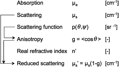
The optical properties of a tissue are described in terms of the absorption coefficient, µa (cm−1), the scattering coefficient µs (cm−1), the scattering function p(θ,ψ) (sr−1) where θ is the deflection angle of scatter and ψ is the azimuthal angle of scatter, and the real refractive index of the tissue, n'. An introduction to these properties is presented elsewhere (Cheong 1995, Jacques and Pogue 2008, Welch and van Gemert 2011).
The p(θ,ψ) is appropriate when discussing only a single or few scattering events, such as during transmission microscopy of thin tissue sections or during confocal reflectance microscopy, which includes optical coherence tomography. In thicker tissues where multiple scattering occurs and the orientations of scattering structures in the tissue are randomly oriented, the ψ dependence of scattering is averaged and hence ignored, and the multiple scattering averages the θ such that an average parameter, g = 〈cos θ〉, called the anisotropy of scatter, characterizes tissue scattering in terms of the relative forward versus backward direction of scatter. Figure 1 summarizes these properties and their inter-relationships.

Figure 1. The optical properties of tissues.
Download figure:
Standard image High-resolution imageOptical scattering can be described either as scattering by particles that have a refractive index different from the surrounding medium, or as scattering by a medium with a continuous but fluctuating refractive index. The particle description can be approximated by Mie theory, which describes the scattering from ideal spheres within a medium (Prahl and Jacques 2012). A mixture of spheres of different sizes can mimic the optical scattering behavior of a tissue. Continuum scattering theory describes tissue scattering in terms of the autocorrelation function for the spatial distribution of the fluctuating refractive index in a tissue (Schmitt and Kumar 1996, Xu and Alfano 2005, Rogers et al 2009, Yi and Backman 2012). The Wiener–Khinchin theorem relates an autocorrelation function to its corresponding power spectrum, and continuum scattering theory relates the spatial autocorrelation of refractive index fluctuations to the wavelength dependence of scatter. Both descriptions are adjusted to match experimental data and hence both are descriptors for the scattering behavior of tissues.
The terms Rayleigh scattering and Mie scattering are commonly used in the field of biomedical optics, with Rayleigh scattering referring to scattering by small particles or mass density fluctuations much smaller than the wavelength of light, and Mie scattering referring to scattering by particles comparable to or larger than the wavelength of light. But this common use of these terms is not actually correct. Mie scattering is the generic name for scattering by a sphere of any size, both small and large, and the common term Rayleigh scattering refers to the Rayleigh limit of Mie scattering due to particles much smaller than the wavelength of light. Nevertheless, the common usage of Rayleigh and Mie is followed in this review because it is familiar to many in our field.
2. The reduced scattering coefficient of tissues
A review of tissue  properties as a function of wavelength is presented, which is not exhaustive but sufficient to characterize the behavior of seven groups of tissues: skin, brain, breast, bone, other soft tissues, other fibrous tissues and fatty tissues. The data of
  (λ) were fit with two equations:

and alternatively

In equation (1), the wavelength λ is normalized by a reference wavelength, 500 nm, to yield a dimensionless value, which is then raised to a power b, called the 'scattering power'. This term characterizes the wavelength dependence of  . The factor a is the value
  (λ = 500 nm), which scales the wavelength-dependent term.
In equation (2), the wavelength dependence of scattering is described in terms of the separate contributions of Rayleigh and Mie scattering at the reference wavelength. The scaling factor a' equals  (λ = 500 nm). The Rayleigh scattering is a'fRay(λ/500 nm)−4, and the Mie scattering is a'(1 – fRay)(λ/500 nm)
 , where 1 – fRay indicates the fraction of Mie scattering.
Table 1 summarizes the parameters of equations (1) and (2) obtained by analysis of the literature data for  (λ). Figure 2 displays the data for each of the seven tissue types. Also shown are the fits to the data using the mean parameters for equations (1) and (2) listed in table 1 for each data set.

Figure 2. Reduced scattering coefficient spectra from the literature for the seven groups of tissues (red circles = data). The green line is the fit using equation (1). The black solid line is the fit using equation (2), with the black dashed lines showing the Rayleigh and Mie components of the fit.
Download figure:
Standard image High-resolution imageTable 1. Parameters specifying thereduced scattering coefficient of tissues: a =  500 nm, such that
  (λ) = a(λ/500 nm)−b, equation (1); aa =
  500 nm, such that
  (λ) = aa(fRay(λ/500 nm)−b + fMie(λ/500 nm)
 ), equation (2); and fMie = 1 – fRay. (na = not available.)
| # | a (cm−1) | b | a' (cm−1) | fRay | bMie | Ref. | Tissue |
|---|---|---|---|---|---|---|---|
| Skin | |||||||
| 1 | 48.9 | 1.548 | 45.6 | 0.22 | 1.184 | Skin | Anderson et al 1982 |
| 2 | 47.8 | 2.453 | 42.9 | 0.76 | 0.351 | Skin | Jacques 1996 |
| 3 | 37.2 | 1.390 | 42.6 | 0.40 | 0.919 | Skin | Simpson et al 1998 |
| 4 | 60.1 | 1.722 | 58.3 | 0.31 | 0.991 | Skin | Saidi et al 1995 |
| 5 | 29.7 | 0.705 | 36.4 | 0.48 | 0.220 | Skin | Bashkatov et al 2011 |
| 6 | 45.3 | 1.292 | 43.6 | 0.41 | 0.562 | Dermis | Salomatina et al 2006 |
| 7 | 68.7 | 1.161 | 66.7 | 0.29 | 0.689 | Epidermis | Salomatina et al 2006 |
| 8 | 30.6 | 1.100 | na | na | na | Skin | Alexandrakis et al 2005 |
| Brain | |||||||
| 9 | 40.8 | 3.089 | 40.8 | 0.00 | 3.088 | Brain | Sandell and Zhu 2011 |
| 10 | 10.9 | 0.334 | 13.3 | 0.36 | 0.000 | Cortex (frontal lobe) | Bevilacqua et al 2000 |
| 11 | 11.6 | 0.601 | 15.7 | 0.53 | 0.000 | Cortex (temporal lobe) | Bevilacqua et al 2000 |
| 12 | 20.0 | 1.629 | 29.1 | 0.81 | 0.000 | Astrocytoma of | Bevilacqua et al 2000 |
| optic nerve | |||||||
| 13 | 25.9 | 1.156 | 25.9 | 0.00 | 1.156 | Normal optic nerve | Bevilacqua et al 2000 |
| 14 | 21.5 | 1.629 | 31.0 | 0.82 | 0.000 | Cerebellar white matter | Bevilacqua et al 2000 |
| 15 | 41.8 | 3.254 | 41.8 | 0.00 | 3.254 | Medulloblastoma | Bevilacqua et al 2000 |
| 16 | 21.4 | 1.200 | 21.4 | 0.00 | 1.200 | Brain | Yi and Backman 2012 |
| Breast | |||||||
| 17 | 31.8 | 2.741 | 31.8 | 0.00 | 2.741 | Breast | Sandell and Zhu 2011 |
| 18 | 11.5 | 0.775 | 15.2 | 0.58 | 0.000 | Breast | Sandell and Zhu 2011 |
| 19 | 24.8 | 1.544 | 24.8 | 0.00 | 1.544 | Breast | Sandell and Zhu 2011 |
| 20 | 20.1 | 1.054 | 20.2 | 0.18 | 0.638 | Breast | Sandell and Zhu 2011 |
| 21 | 14.6 | 0.410 | 18.1 | 0.41 | 0.000 | Breast | Spinelli et al 2004 |
| 22 | 12.5 | 0.837 | 17.4 | 0.60 | 0.076 | Breast, premenopausal | Cerussi et al 2001 |
| 23 | 8.3 | 0.617 | 11.2 | 0.54 | 0.009 | Breast, postmenopausal | Cerussi et al 2001 |
| 24 | 10.5 | 0.464 | 10.5 | 0.00 | 0.473 | Breast | Durduran et al 2002 |
| Bone | |||||||
| 25 | 9.5 | 0.141 | 9.7 | 0.04 | 0.116 | Skull | Bevilacqua et al 2000 |
| 26 | 20.9 | 0.537 | 20.9 | 0.00 | 0.537 | Skull | Firbank et al 1993 |
| 27 | 38.4 | 1.470 | na | na | na | Bone | Alexandrakis et al 2005 |
| Other soft tissues | |||||||
| 28 | 9.0 | 0.617 | 11.5 | 0.61 | 0.000 | Liver | Parsa et al 1989 |
| 29 | 13.0 | 0.926 | 13.0 | 0.00 | 0.926 | Muscle | Tromberg 1996 |
| 30 | 12.2 | 1.448 | 13.0 | 0.44 | 0.731 | Fibroadenoma breast | Peters et al 1990 |
| 31 | 18.8 | 1.620 | 18.8 | 0.00 | 1.620 | Mucous tissue | Bashkatov et al 2011 |
| 32 | 28.1 | 1.507 | 27.7 | 0.23 | 1.165 | SCC | Salomatina et al 2006 |
| 33 | 42.8 | 1.563 | 42.5 | 0.10 | 1.433 | Infiltrative BCC | Salomatina et al 2006 |
| 34 | 31.9 | 1.371 | 31.5 | 0.15 | 1.157 | Nodular BCC | Salomatina et al 2006 |
| 35 | 16.5 | 1.240 | na | na | na | Bowel | Alexandrakis et al 2005 |
| 36 | 14.6 | 1.430 | na | na | na | Heart wall | Alexandrakis et al 2005 |
| 37 | 35.1 | 1.510 | na | na | na | Kidneys | Alexandrakis et al 2005 |
| 38 | 9.2 | 1.050 | na | na | na | Liver&spleen | Alexandrakis et al 2005 |
| 39 | 25.4 | 0.530 | na | na | na | Lung | Alexandrakis et al 2005 |
| 40 | 9.8 | 2.820 | na | na | na | Muscle | Alexandrakis et al 2005 |
| 41 | 19.1 | 0.970 | na | na | na | Stomach wall | Alexandrakis et al 2005 |
| 42 | 22.0 | 0.660 | na | na | na | Whole blood | Alexandrakis et al 2005 |
| 43 | 16.5 | 1.640 | 16.5 | 0.00 | 1.640 | Liver | Yi and Backman 2012 |
| 44 | 8.1 | 0.980 | 8.1 | 0.00 | 0.980 | Lung | Yi and Backman 2012 |
| 45 | 8.3 | 1.260 | 8.3 | 0.00 | 1.260 | Heart | Yi and Backman 2012 |
| Other fibrous tissues | |||||||
| 46 | 33.6 | 1.712 | 37.3 | 0.72 | 0.000 | Tumor | Sandell and Zhu 2011 |
| 47 | 30.1 | 1.549 | 30.1 | 0.02 | 1.521 | Prostate | Newman and Jacques 1991 |
| 48 | 27.2 | 1.768 | 29.7 | 0.61 | 0.585 | Glandular breast | Peters et al 1990 |
| 49 | 24.1 | 1.618 | 25.8 | 0.49 | 0.784 | Fibrocystic breast | Peters et al 1990 |
| 50 | 20.7 | 1.487 | 22.8 | 0.60 | 0.327 | Carcinoma breast | Peters et al 1990 |
| Fatty tissue | |||||||
| 51 | 13.7 | 0.385 | 14.7 | 0.16 | 0.250 | Subcutaneous fat | Simpson et al 1998 |
| 52 | 10.6 | 0.520 | 11.2 | 0.29 | 0.089 | Adipose breast | Peters et al 1990 |
| 53 | 15.4 | 0.680 | 15.4 | 0.00 | 0.680 | Subcutaneous adipose | Bashkatov et al 2011 |
| 54 | 35.2 | 0.988 | 34.2 | 0.26 | 0.567 | Subcut. fat | Salomatina et al 2006 |
| 55 | 21.6 | 0.930 | 21.1 | 0.17 | 0.651 | Subcut. adipocytes | Salomatina et al 2006 |
| 56 | 14.1 | 0.530 | na | na | na | Adipose | Alexandrakis et al 2005 |
Table 2 summarizes the mean values of the parameters for equations (1) and (2) as applied to each of the seven tissue types in table 1.
Table 2. Average parameters for reduced scattering coefficient,  , for tissues.
| a (cm−1) | b | a' (cm−1) | fRay | bMie | |
|---|---|---|---|---|---|
| Skin | |||||
| Mean | 46.0 | 1.421 | 48.0 | 0.409 | 0.702 |
| SD | 13.7 | 0.517 | 10.6 | 0.178 | 0.351 |
| n | 8 | 8 | 7 | 7 | 7 |
| Brain | |||||
| Mean | 24.2 | 1.611 | 27.4 | 0.315 | 1.087 |
| SD | 11.7 | 1.063 | 10.5 | 0.368 | 1.386 |
| n | 8 | 8 | 8 | 8 | 8 |
| Breast | |||||
| Mean | 16.8 | 1.055 | 18.7 | 0.288 | 0.685 |
| SD | 8.1 | 0.771 | 7.0 | 0.273 | 0.984 |
| n | 8 | 8 | 8 | 8 | 8 |
| Bone | |||||
| Mean | 22.9 | 0.716 | 15.3 | 0.022 | 0.326 |
| SD | 14.6 | 0.682 | 7.9 | 0.032 | 0.298 |
| n | 3 | 3 | 2 | 2 | 2 |
| Other soft tissues | |||||
| Mean | 18.9 | 1.286 | 19.1 | 0.153 | 1.091 |
| SD | 10.2 | 0.521 | 11.3 | 0.216 | 0.483 |
| n | 18 | 18 | 10 | 10 | 10 |
| Other fibrous tissues | |||||
| Mean | 27.1 | 1.627 | 29.2 | 0.489 | 0.644 |
| SD | 5.0 | 0.115 | 5.4 | 0.274 | 0.572 |
| n | 5 | 5 | 5 | 5 | 5 |
| Fatty tissue | |||||
| Mean | 18.4 | 0.672 | 19.3 | 0.174 | 0.447 |
| SD | 9.0 | 0.242 | 9.1 | 0.111 | 0.263 |
| n | 6 | 6 | 5 | 5 | 5 |
So which is better, equation (1) or equation (2)? The equations are equally good for routine prediction of tissue scattering for use in predicting behavior of light diffusion within the 400–1300 nm wavelength range. But outside this range in either the ultraviolet or the longer infrared, the two equations diverge. More data is needed, especially at longer wavelengths, to resolve which equation is better.
The bigger issue is the variability of the a and a' values, which scale the wavelength-dependent terms in equations (1) and (2). In particular, the category 'other soft tissues' show significant variability in a and a'. Figure 3 ranks the data according to the value of a in equation (1), showing that skin and other fibrous tissues have higher values of a ( 500 nm) than other tissues. Breast tissues are seen at both low and high scattering, perhaps dependent on the relative fibrous versus fatty character of the particular breast.

Figure 3. Ranking the tissues by their scattering at 500 nm,  500 nm, specified by the parameter a in equation (1). The numbers in parentheses indicate the # in table 1.
Download figure:
Standard image High-resolution imageIf one is interested in using the scattering properties to characterize the sub-µm structure of a cell, then the details of equations (1) and (2) become important. In general, cellular tissues will present a simple λ−b behavior, and equation (1) is sufficient. Cellular tissues with a high density of mitochondria (Beauvoit et al 1995) or lysosomes (Wilson et al 2007) will present Rayleigh scattering due to the high density of lipid membranes, which causes an elevation of b in equation (1) and an elevation of fRay in equation (2). Collagenous tissues, such as skin and some fibrous tissues, present much more Rayleigh scattering putatively due to the 70 nm periodic density along collagen fibrils and the sub-100 nm inter-fibril spacings (Saidi et al 1995, Jacques 1996), which also elevates b and fRay.
Figure 4(a) plots bMie versus b, and shows some tissues tracking as bMie = b, while other tissues, especially the skin and fibrous tissues, show a lower bMie than b. When the data allow specification of both a short wavelength rise and a long wavelength stability in  , then fRay can account for the Rayleigh scattering and bMie can account for the slower fall in
  versus longer wavelengths. Figure 4(b) shows the ratio bMie/b versus fRay, illustrating the drop in bMie relative to b as fRay grows.
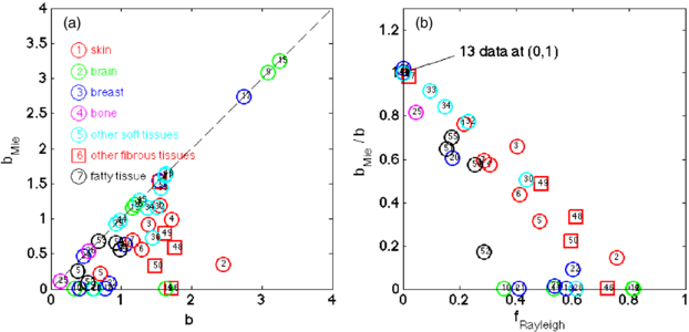
Figure 4. (a) Plot of bMie versus b in equations (2) and (1), respectively. (b) Plot of bMie/b versus fRayleigh. The data are from table 1. When fRayleigh is significant, bMie is less than b.
Download figure:
Standard image High-resolution imageMore data, especially at longer wavelengths, is needed to clarify if Mie scattering is indeed relatively wavelength independent (bMie ≤ 1). If so, then equation (2) is a better descriptor than equation (1), and the short wavelength rise in  specifies an fRay that becomes a useful parameter for quantifying the scattering due to organelles and collagen fibrils. If not, then the entire spectrum is consistent with equation (1) and the simple a(λ/λreference)−b behavior implies the corresponding autocorrelation of refractive index fluctuations (i.e. mass fluctuations) follows a simple form. Whether one form or the other is more useful remains to be seen. This question is an area of study that hopes to use changes in the structure of cells and tissues in the ∼50–600 nm range as a contrast parameter while imaging cells or tissues macroscopically. Such surveillance may prove useful in imaging the margins of cancers, for example.
3. Scattering µs and anisotropy g
The measurement of µs can be a difficult task. The measurement of µs is usually made by a collimated transmission measurement (Tc) through tissue of thickness L to specify µs = –ln(Tc)/L. But such measurements must be made through a thin tissue sample, on the scale of one mean free path (mfp = 1/µs), which is typically 100 µm or less, or else multiple scattering becomes an issue. But preparing such thin tissues is not easy, and they are subject to desiccation. Also, the heterogeneity of tissues becomes apparent in such thin samples. Another issue is the solid angle of collection at the detector, which if too large will collect photons despite their being slightly deflected, thereby underestimating µs.
Similarly, the measurement of g can be difficult. Direct measurement of p(θ) using goniometry involves measurement of the angular scattering of light by a thin tissue sample, which then allows calculation of g (see below). The concerns about local heterogeneity in a thin sample pertain to goniometry. Also, the measurements in the backward direction are often low, and must be well above any noise floor of measurement since the backward signal is critical to the net value of g. When measuring a thin tissue slab, the angle and intensity of exit from the tissue can be modified by refraction at the tissue/air or tissue/glass/air interface. Using a hemispherical lens coupled to the tissue allows exiting photons to encounter a glass/air interface perpendicularly, which mitigates refraction. Measurements of scattering around θ = 90 can be experimentally complicated.
One approach toward measuring g is to use the values of  from diffuse light measurements and µs from collimated transmission measurements to deduce g: g = 1 –
  /µs. While the
  value is usually robust, the µs value may not be so reliable, as discussed above. An artifactual decrease in µs causes an artifactual decrease in g.
A recent approach (Gareau 2006, Samatham et al 2008, Jacques et al 2008) has been to measure the attenuation of backscattered reflectance collected by a confocal microscope as the focus is scanned down into a tissue. A high g value allows light to penetrate to the focus despite multiple scattering, and to return from the focus and still reach the pinhole of collection. However, a high g value reduces the amount of light backscattered at the focus which decreases the collected reflectance. The measurement of reflectance, R(zf) = ρ exp(–µzf), depends on two parameters, (1) the attenuation (µ (cm−1)) versus depth of focus and (2) the absolute value of reflected signal within the focus (ρ, a mirror defines ρ = 1). Together, µ and ρ specify the two unknown values µs and g.
Figure 5(a) shows the measurements at 488 nm wavelength of Samatham (2012) on freshly excised mouse tissues, illustrating how µ and ρ specify µs and g. Figure 5(b) plots µs versus g as well as iso- contours. The data show that µs and g increase coordinately, while µs(1 – g) remains somewhat constant in the range of 30–50 cm−1.
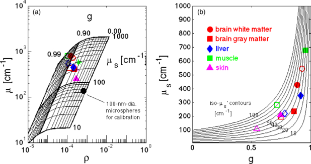
Figure 5. Scattering coefficient µs versus anisotropy g at 488 nm wavelength. (a) Experimental confocal reflectance data of attenuation (µ (cm−1)) versus depth of focus and absolute value of reflected signal (ρ, a mirror defines ρ = 1) (Samatham 2012). Grid shows the expected values of µ, ρ for various µs, g values. Open symbols are tissues exposed to saline. Closed symbols are tissues not directly contacted by saline, but kept moist via vapor pressure. (b) Plot of µs versus g using values specified in figure 4(a). Several iso- contours are drawn, with tissues mostly in the range of 30–50 cm−1.
Download figure:
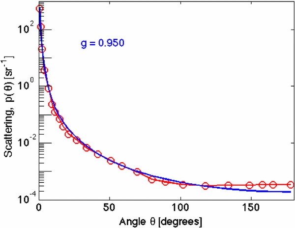
Standard image High-resolution imageMourant et al (2002) reported on the scattering properties of cultured cells in suspension. Figure 6 shows the scattering function p(θ) (sr−1) for light polarized perpendicular to the scattering plane (p(θ)per) and for light polarized parallel to the scattering plane (p(θ)par). The scattering plane is defined as the plane containing the laser source, cell sample and the detector. The forward scattering is denoted by θ = 0°, and direct backscatter is denoted by θ = 180°. The cells show a very forward-directed scatter, with anisotropies of g = 0.925, 0.950 and 0.930 for the perpendicular, parallel and total scattering functions (arccos(0.925) = 22.3°, arccos(0.950) = 18.2° and arccos(0.930) = 21.6°).

Figure 6. Angular scattering function, p(θ) (sr−1), of cells in suspension (androgen-independent malignant rat prostate carcinoma cells). The data are taken from Mourant et al (2002), and plotted after normalizing so that equation (6) holds for p(θ)tot = 0.5(p(θ)per + p(θ)par). The p(θ)per and p(θ)par are the scattering for polarized light oriented perpendicular and parallel to the scattering plane (see text). The anisotropies of scattering, g, are indicated for each curve. The green line is the Henyey–Greenstein function for g = 0.930, which is the g value for the total scattering, showing an approximation to the cellular scattering.
Download figure:
Standard image High-resolution imageXu et al (2008) reported on the angular and wavelength dependence of the scattering function p(θ, λ). Figure 7 shows the p(θ) for their cells (SiHa cells in phosphate buffered saline suspensions) at 633 nm wavelength. Their report is especially interesting because they demonstrated that the first 10° of angular deflection are dominated by the cell as a whole and by the nucleus, consistent with Mie scattering from large spheres. At wider angles >10°, the scattering was due to the small-scale refractive index fluctuations of the organelles, aggregates and membranes of the cell, and this broad scattering was modeled by a continuum model.

Figure 7. Angular scattering function, p(θ) (sr−1), of cells at 633 nm wavelength. Data from Xu et al (2008). The blue line is a Henyey–Greenstein fit to the data. The p(θ) function has been properly normalized to satisfy equation (6).
Download figure:
Standard image High-resolution imageJacques et al (1987) and Hall et al (2012) studied the goniometry of light transmission through tissues of varying sample thickness. The scattered light could be described by an equivalent Henyey–Greenstein function with an apparent g. As the tissue thinned, this apparent g value extrapolated toward the expected g value for a single-scattering Henyey–Greenstein function. These reports cited values of g greater than 0.90 for visible wavelengths (see figure 8). This method offers an approach toward direct measurement of p(θ) by goniometry using thicker samples.

Figure 8. The anisotropy of scattering versus wavelength.
Download figure:
Standard image High-resolution imageFigure 8 plots literature data on anisotropy versus wavelength. There is a lot of variation in the data, but in general the values of g are rather high. There appears to be a trend toward increasing g as the wavelength increases. This observation, if true, is surprising. If the small sub-wavelength structures within a cell are scattering light, then as the wavelength increases the ratio of structure size to wavelength should decrease, and the scattering should become more Rayleigh-like, i.e. lower g. Why does g increase with increasing λ? This contradiction between experiment and expectation is an opportunity to better understand the nature of light scattering in tissues. Perhaps the Mie scattering from the nuclei dominates in certain experiments, which keeps g high. Perhaps there is some mesoscopic scale of structure in tissue, ≫10 µm, that generates constructive interference so that more light is forward-scattered and hence g increases. The efficiency of the smallest scatterers decreases as λ increase, and perhaps their contribution to the apparent g simply diminishes, yielding a higher g at longer wavelengths. Because of the importance of g in microscopy and interferometry, more studies on anisotropy should be a priority.
4. The refractive index, n
The complex refractive index, n = n' + jn'', includes the real refractive index, n', which describes energy storage and hence affects the speed of light in a medium. The imaginary refractive index, n'', describes energy dissipation and specifies the absorption coefficient, µa = 4πn''/λ. To a first approximation, the value of n' scales as the water content (W) of a tissue.

where  is the refractive index of the tissue's dry mass and
  is the refractive index of water. Jacques and Prahl (1987) estimated that
  = 1.33 and
  = 1.50, based on an old Bausch and Lomb graphic that had plotted n' versus water content for various biological materials and food products. A more recent report by Biswas and Luu (2011) on a range of biological tissues used magnetic resonance imaging (MRI) to indicate that ρdry = 1.53 g cm−3 and
  = 1.514. Figure 9 summarizes their data illustrating this relationship.

Figure 9. The real refractive indexof biological tissues, measured with an Abbé refractometer, versus the density (g cm−3) (data from table in Biswas and Luu (2011)). The authors used MRI to determine the water content (W), which suggested the dry mass density was ρdry = 1.53 g cm−3. Using this value, the relationship n' versus W can be specified, as in equation (3).
Download figure:
Standard image High-resolution image5. Absorption coefficient µa
A light-absorbing medium will absorb a fraction of incident light per incremental pathlength of travel within the medium. The absorption coefficient µa (cm−1) is defined as

where T (dimensionless) is the transmitted or surviving fraction of the incident light after an incremental pathlength ∂L (cm). This fractional change ∂T/T per ∂L yields an exponential decrease in the intensity of the light as a function of increasing pathlength L:

Equation (5) also cites two alternative expressions using alternative descriptors for absorption. The first spectrometers measured the transmission through a nonscattering medium containing a chromophore as T = 10−εCL, where C is the concentration ((mol L−1) or (M)) and ε is the extinction coefficient (cm−1 M−1) for the chromophore. Historically, ε has been recorded in the literature using this base 10 nomenclature. Optical wave theory describes transmission of intensity as T = exp(–4πn''L/λ), where n'' is the imaginary refractive index of the medium, hence µa = 4πn''/λ. You can find the absorption of a chromophore recorded in these three different ways, ε, µa and n'', but they are equivalent descriptors.
The absorption coefficient µa of a tissue is the sum of contributions from all absorbing chromophores within the tissue:

For example, consider HGb. The HGb mass concentration within blood, Cm.HGb (g L−1), varies for men (138 to 172 g L−1), women (121 to 151 g L−1), children (110 to 160 g L−1) and pregnant women (110 to 120 g L−1) (Tresca 2012). But the blood volume fraction (B) in a tissue also varies. The molecular weight of HGb is MW = 64 458 g mol−1 (van Beekvelt et al 2001). If B = 0.01 and Cm.HGb = 150 g L−1, then the apparent average HGb molar concentration in the tissue is CHGb = BCm.HGb/MW = (0.01)(150 g L−1)/(64 458 g mol−1) = 2.33 × 10⁻⁵ M. The extinction coefficient of HGb varies with its oxygen saturation and with wavelength. At the isobestic point at ∼806 nm, both oxyHGb and deoxyHGB have the same absorption, and the value of ε is ∼818 cm−1 M−1. At 806 nm, the contribution of blood (B = 0.01) to the tissue absorption is µa = ln(10)CHGbε = (2.302)(2.33 × 10⁻⁵ M)(818) = 0.0438 cm−1.
Sometimes one wishes to describe the absorption properties of a material that does not have a well defined concentration, and an alternative concentration must be used, for example, C (mg mL−1), and an alternative extinction coefficient must be used, ε (cm−1 (mg mL−1)−1). The product εC still has units of cm−1, and εCL is dimensionless. So, while the literature usually uses C (M), ε (cm−1 M−1) and L (cm), alternative units for C, ε and L may be used, as long as εCL is dimensionless.
Studies on tissue optical properties will usually cite values of a tissue's average absorption coefficient µa, since the molecular composition of the tissue is not well specified. It is convenient to modify equation (6) so that the equation uses the volume fraction of a tissue component (fv.i (L L−1) or (dimensionless)) and the absorption coefficient of that pure component (µa.i (cm−1)). Using this approach, equation (6) can be rewritten as

For example, sometimes it is helpful to describe the apparent blood volume fraction B in a tissue rather than citing an average CHGb in the tissue. Citing B conveys a more anatomical sense of the density of vasculature. If one adopts the convention followed by Prahl (2012a) of assigning whole blood the HGb mass concentration Cm.HGb = 150 g L−1, then in equation (7) the fv.blood would equal B. The µa.blood would equal εbloodln(10)Cm.HGb/MW = εbloodln(10) (150 g L−1)/(64 458 g mol−1) = 0.0536εblood, where εblood varies with wavelength. At the isobestic point εblood = 818 cm−1, as above, and the value of µa.blood becomes 4.38 cm−1. If a tissue has an average volume fraction (fv.blood = B = 0.01) of blood, then the blood contribution to µa equals (0.01)(4.38 cm−1) = 0.0438 cm−1.
Another example is water content. The imaginary refractive index of water at 970 nm is n'' = 3.47 × 10⁻⁶. The absorption coefficient of water at λ = 970 nm is µa.water = 4πn''/λ = 0.45 cm−1. If a tissue has a volume fraction of water fv.water = 0.65, then the contribution of water to the total tissue absorption at 970 nm is µa = fv.waterµa.water = (0.65)(0.45 cm−1) = 0.29 cm−1.
There are a variety of chromophores, both natural and exogenously supplied, which can contribute to µa in equation (6) or (7). Usually, blood and water will dominate the absorption. Sometimes, melanin, fat, bilirubin, beta-carotene or an additive such as indocyanine green must be considered. Other chromophores offer quite minor contributions. If one is interested in spectroscopic detection, then the minor contributions are important. If one is interested in understanding light penetration into a tissue for some therapeutic protocol, then the minor contributions usually do not significantly perturb the light transport.
5.1. Blood
The absorption coefficient of whole blood is shown in figure 10, using data compiled by Prahl (2012a), citing data from Gratzer and Kollias (1999), Moaveni (1970), Schmitt (1986) Takatani and Graham (1987). Figure 10(a) shows fully oxygenated blood, and figure 10(b) shows fully deoxygenated blood. Reliable data beyond 1000 nm wavelength is difficult to find in the literature. In figure 10, dashed red lines extrapolate data beyond 1000 nm, either using a Gaussian or an exponential, indicating where water absorption might begin to dominate over HGb absorption.
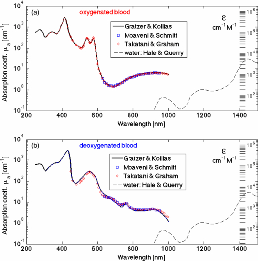
Figure 10. Absorption coefficient of whole blood versus wavelength. (Data from Prahl (2012a), citing data from Gratzer and Kollias (1999), Moaveni (1970), Schmitt (1986), Takatani and Graham (1987).) Dashed red lines extrapolate data beyond 1000 nm, either using a Gaussian or an exponential, indicating where water absorption might begin to dominate over HGb absorption. (a) Oxygenated whole blood. (b) Deoxygenated whole blood.
Download figure:
Standard image High-resolution image5.2. Water
The water absorption spectrum is plotted in figure 11(a), based on the work of Hale and Querry (1973), Zolotarev et al (1969) and Segelstein (1981), as cited on the website by Prahl (2012b). Figure 11(b) shows the difference between free water and bound water reported by Chung et al (2012), in which the absorption of bound water slightly sharpens the absorption peak at about 970 nm, i.e., absorption of bound water decreases above and below 970 nm relative to free water.

Figure 11. Absorption coefficient of water versus wavelength. (a) Data from Hale and Querry (1973), Zolotarev et al (1969) and Segelstein (1981). (b) Data on free versus bound water from Chung et al (2012), showing the drop in absorption above and below the peak at about 970 nm for bound water.
Download figure:
Standard image High-resolution imageIf interested in water absorption during exposure to high energy laser pulses, the report of Cummings and Walsh (1993) discusses how the mid-infrared water absorption near 3 µm wavelength broadens and the peak absorption decreases as the pulsed laser energy deposition (J cm−3) in the water increases.
5.3. Melanin
The absorption coefficient of the interior of a typical cutaneous melanosome, µa.melanosome (cm−1), is shown in figure 12 (open black symbols), based on the work of Jacques and McAuliffe (1991). In that report, the threshold radiant exposure, H (J cm−3), of a ruby laser (690 nm wavelength) for causing explosive vaporization of melanosomes within cadaver skin was tested as a function of initial tissue temperature. A colder initial temperature required a higher laser pulse energy to pop the melanosomes. The results predicted the threshold temperature for explosive vaporization to be 112 °C. This value was used to interpret the literature of reported values of threshold H for exploding cutaneous melanosomes using a variety of lasers at various wavelengths. The analysis yielded the µa for the interior of cutaneous melanosomes. The resulting spectrum was consistent with optical fiber spectra for the ventral versus sun-exposed dorsal forearm skin of subjects; the difference in optical density attributed to cutaneous melanin (red circles, scaled to match laser results). The figure also shows the optical fiber probe measurements of Zonios et al (2008), again scaled to match laser results. The data of Sarna and Swartz (1988) specified the extinction coefficient ε (cm−1 M−1) of monomers for eumelanin and pheomelanin. In figure 11, these data are scaled by an intra-melanosome concentration of 461 mM for eumelanin monomers and 564 mM for pheomelanin monomers, in order to match the µa.melanosome spectra at 500 nm. The fits use a power curve,

where the value 519 cm−1 at 500 nm was specified by the laser experiments. The value of the power factor m cited by different reports varies as shown in the figure, and an approximate value for m is 3. More work on the absorption spectrum of in vivo melanin is needed.
To calculate the µa contribution for melanin in a tissue, one estimates the equivalent volume fraction (fv.melanosome) of cutaneous-like melanosomes within a tissue, fv.melanin, which is then multiplied by this µa.melanosome to yield the contribution to the total µa of a tissue:

Using fv.melanosome as a concentration of melanin may seem odd, but melanin is an extended polymer that does not have a unique molecular weight. Also, histology can document the number density of melanosomes in a tissue, so using fv.melanosome is perhaps a more familiar metric to some people, such as pathologists. However, melanosomes do not all have the same melanin content. The µa.melanosome of figure 12 is for a typical cutaneous melanosome, predominantly eumelanin, used as a convention. The figure shows the difference between eumelanin (black) and pheomelanin (red).

Figure 12. Absorption coefficient of the interior of a typical cutaneous melanosome versus wavelength, µa.melanosome (cm−1).
Download figure:
Standard image High-resolution imageAlternatively, one can cite the apparent concentration of monomers (Ceumelanin and Cpheomelanin (M)) in a tissue and use the extinction coefficients of Sarna and Swartz (1988),

such that the absorption due to melanin is

5.4. Adipose tissue and fat
The absorption coefficient spectra of several fatty tissues are shown in figure 13. The work of van Veen et al (2004) involved careful purification and dehydration of porcine fat before measurement, and perhaps is the best spectra available at this point. Other measurements are on tissues of unknown fat and water content. An attempt to correct for the fat and water content has been made, and the spectra are in general agreement that the dominant absorption peak is at 930 nm.

Figure 13. Absorption coefficient of fatty tissues versus wavelength. The pig fat spectrum of van Veen et al (2004) was highly purified. The other spectra have been corrected for fat content and corrected for the absorption by water, but the corrections are not perfect.
Download figure:
Standard image High-resolution image5.5. Yellow pigments
The yellow pigments, bilirubin and β-carotene, are sometimes present to a small degree in the absorption spectra of tissues. Bilirubin absorption in the skin is routinely used to detect hyperbilirubinemia in neonates. β-carotene can also give a yellow hue to tissues. Figure 14 cites the extinction coefficient for bilirubin and β-carotene. Dr Angelo Lamola provided the spectrum of bilirubin associated with albumin in human serum (bilirubin/HSA) (Lamola 2011). A report of bilirubin in chloroform is also shown (Du et al 1998), illustrating the solvent effect on absorption. The β-carotene spectrum in a solvent, hexane, is shown (Du et al 1998) and the in vivo value is expected to differ slightly.

Figure 14. The extinction coefficient of bilirubin (in chloroform or bound to human serum albumin) and β-carotene (in hexane) (Du et al 1998, Lamola 2011).
Download figure:
Standard image High-resolution image6. A generic tissue
The optical properties of tissues should be regarded as variable from tissue to tissue, person to person and even time to time. Methods for measuring optical properties continue to improve and it is feasible to make rapid assessment of a particular tissue, much like taking a temperature with a thermometer.
For the reader who wishes to estimate optical properties to guide device or protocol design, a generic tissue can be constructed that is specified by the absorbing chromophores in the tissue and by the balance of Rayleigh and Mie scattering in the tissue.
Figure 15 shows the absorption coefficient µa increasing as water, blood, bilirubin, fat and melanin are sequentially added. This figure does not describe a real tissue, but simply illustrates the spectral consequence of the various absorbing chromophores. Any tissue can be characterized by
- S HGb oxygen saturation of mixed arterio-venous vasculature
- B average blood volume fraction (fv.blood)
- W water content (fv.water)
- Bili bilirubin concentration (C (M))
- βC β-carotene concentration (C (M))
- F fat content (fv.fat)
- M melanosome volume fraction (fv.melanosome), or alternatively the molar concentration of melanin monomers (C (M)).
The total absorption coefficient is calculated

Figure 16 shows a more realistic tissue, in which the blood content is fixed at B = 0.002, S = 0.75, and there is a baseline volume fraction of fibrous material, fv.fibrous = 0.30. The tissue fat content and water content offset each other, with F = [0 by 0.1 to 0.7] as W = [0.7 by −0.1 to 0.1] such that fat + water = 0.70. The fat signature is evident at water contents below 30, but is less obvious at higher water contents.

Figure 15. Total absorption coefficient µa (cm−1), as water is added (volume fraction fv.water = 0.1 by 0.1 to 0.9), blood at 75 oxygen saturation is added (average fv.blood = 10−4 by 10−4 to 2 × 10⁻³), bilirubin is added (1 by 1 to 20 mg dL−1, where 20 mg dL−1 = 342 µM is a bilirubin concentration in the blood of a jaundiced neonate), fat is added (fv.fat = 0.3 by 0.3 to 0.9), and melanin is added (fv.melanosome = 0.01 by 0.01 to 0.10).
Download figure:
Standard image High-resolution image
Figure 16. The absorption spectrum of a tissue (B = 0.002, S = 0.75, fv.fibrous = 0.30) that varies its water content from 0 by 0.1 to 0.7 as the fat content varies from 0.7 by 0.1 to 0, such that fat + water = 0.7. Magenta lines are for high fat, low water, and the fat signature is clearly present at 930 nm (arrow). The blue lines are for low fat, high water (W ≥ 0.3), and the fat signature is less obvious. (Based on the fat spectrum of van Veen et al (2004).)
Download figure:
Standard image High-resolution imageFigure 17 shows the generic reduced scattering coefficient of tissues, based on equation (2). The contribution of Mie scattering (aMie) is shown as blue lines. The contribution of Rayleigh scattering (aRayleigh) is added to the highest Mie scattering, and the combination is shown as red lines (aRayleigh + aMie). As the Rayleigh component of scattering increases, the short wavelength scattering increases significantly.

Figure 17. Generic scattering. The reduced scattering coefficient,  (cm−1), of a generic tissue, with variable contributions from Rayleigh and Mie scattering. The contribution of Mie scattering is shown as blue lines (aMie = 5 to 20 cm−1, aRayleigh = 0). The Rayleigh scattering (aRayleigh = 5 to 60 cm−1, aMie = 20 cm−1) plus Mie scattering is shown as red lines (aRayleigh + aMie).
Download figure:
Standard image High-resolution image
Equations (1), (2) and (6), (7) can mimic the optical properties of a generic tissue at any wavelength, but one must specify the tissue parameters in these equations. The literature is limited in its reporting of in vivo optical properties. The task now is to better understand the constitution of tissues in terms of tissue chromophores and tissue parameters that govern absorption to enable use of the generic model. Table 3 lists a brief survey of the in vivo optical parameters that affect absorption (CHGb, B, S, W, M, F).
Table 3. In vivo tissue parametersgoverning optical absorption. CHGb = total HGb concentration (µM), B = blood volume fraction × 100% (assuming 150 g HGb L−1 blood), S = oxygen saturation of HGb × 100%, W = water volume fraction × 100%, M = melanosome volume fraction × 100%. Human tissues unless otherwise labeled. (na = not available.)
| Tissue (reference) | CHGb (µM) | B% | S% | W% | F% | M% |
|---|---|---|---|---|---|---|
| 1 Breast, normal (Tromberg et al 1997) | 23.6 | 1.02 | 67.6 | 14.4 | 65.6 | 0 |
| 2 Breast, normal (Bevilacqua et al 2000) | 24.2 | 1.04 | 75.5 | 29.2 | 51.7 | 0 |
| 3 Breast, normal (Durduran et al 2002) | 34.0 | 1.46 | 68.0 | na | na | 0 |
| 4 Breast, normal (Jakubowski et al 2004) | 16.0 | 0.69 | 62.6 | 6.0 | 74.0 | 0 |
| 5 Breast, normal (Spinelli et al 2004) | 15.7 | 0.67 | 66.4 | 14.5 | 58.0 | 0 |
| 6 Breast, tumor (Jakubowski et al 2004) | 41.0 | 1.76 | 61.1 | 41.0 | 39.0 | 0 |
| 7 Abdomen (Jakubowski et al 2004) | 12.5 | 0.54 | 76.0 | 11.0 | 69.0 | 0 |
| 8 Dermis (Choudhury et al 2010) | 4.7 | 0.20 | 39.0 | 65.0 | 0 | 0 |
| 9 Epidermis (Choudhury et al 2010) | 0 | 0 | 0 | na | na | 2.50 |
| 10 Skin I–II (500–600 nm) (Tseng et al 2011) | 1.1 | 0.05 | 75.7 | na | na | 1.65 |
| 11 Skin I–II (600–1000 nm) (Tseng et al 2011) | 7.9 | 0.34 | 98.5 | 21.4 | 27.7 | 0.87 |
| 12 Skin III–IV (500–600 nm) (Tseng et al 2011) | 8.2 | 0.35 | 96.2 | na | na | 1.98 |
| 13 Skin III–IV (600–1000 nm) (Tseng et al 2011) | 9.6 | 0.41 | 99.2 | 26.1 | 22.5 | 1.15 |
| 14 Skin V–VI (600–1000 nm) (Tseng et al 2011) | 2.7 | 0.12 | 99.3 | 16.6 | 18.7 | 1.65 |
| 15 Forearm (Matcher et al 1997) | 117.0 | 5.03 | 64.1 | na | na | na |
| 16 Head (Matcher et al 1997) | 78.0 | 3.35 | 64.1 | na | na | na |
| 17 Calf (Matcher et al 1997) | 84.0 | 3.61 | 69.0 | na | na | na |
| 18 Neonatal brain (Zhao et al 2004) | 39.7 | 1.71 | 58.7 | na | na | 0 |
| 19 Neonatal brain (Ijichi et al 2005) | 64.7 | 2.78 | 70.0 | na | na | 0 |
| 20 Prostate (Svensson 2007) | 215.0 | 9.24 | 76.0 | na | na | 0 |
| 21 Canine bowel (Solonenko et al 2002) | 119.0 | 5.11 | 80.0 | na | na | 0 |
| 22 Canine kidney (Solonenko et al 2002) | 340.0 | 14.61 | 70.0 | na | na | 0 |
| 23 Canine prostate (Solonenko et al 2002) | 51.0 | 2.19 | 50.0 | na | na | 0 |
| 24 Canine myocardium (Eliasen et al 1982) | 100.1 | 4.30 | na | na | na | 0 |
| 25 Rat brain cortex (Todd et al 1992) | 58.2 | 2.50 | na | na | na | 0 |
| 26 Rat brain cortex (Abookasis et al 2009) | 87.3 | 3.75 | 60.7 | na | na | 0 |
| 27 Rat brain cortex normal (O'Sullivan et al 2012) | 71.0 | 3.05 | 59.0 | na | na | 0 |
| 28 Rat brain cortex occluded (O'Sullivan et al 2012) | 65.0 | 2.79 | na | na | na | 0 |
| 29 Sheep&horse brain (Weaver et al 1989) | 32.9 | 1.42 | na | na | na | 0 |
| 30 Sheep&horse heart (Weaver et al 1989) | 160.6 | 6.90 | na | na | na | 0 |
| 31 Sheep&horse lung (Weaver et al 1989) | 1355.5 | 58.25 | na | na | na | 0 |
| 32 Sheep&horse liver (Weaver et al 1989) | 1151.9 | 49.50 | na | na | na | 0 |
| 33 Sheep&horse kidney (Weaver et al 1989) | 723.7 | 31.10 | na | na | na | 0 |
| 34 Sheep&horse small intestine (Weaver et al 1989) | 214.1 | 9.20 | na | na | na | 0 |
| 35 Sheep&horse large intestine (Weaver et al 1989) | 151.3 | 6.50 | na | na | na | 0 |
| 36 Sheep&horse muscle (Weaver et al 1989) | 27.0 | 1.16 | na | na | na | 0 |
| 37 Sheep&horse tongue (Weaver et al 1989) | 216.4 | 9.30 | na | na | na | 0 |
| 38 Sheep&horse skin (Weaver et al 1989) | 36.4 | 1.57 | na | na | na | 0 |
| 39 Sheep&horse subcut. fat (Weaver et al 1989) | 17.7 | 0.76 | na | na | na | 0 |
| 40 Sheep&horse omental fat (Weaver et al 1989) | 60.7 | 2.61 | na | na | na | 0 |
| 41 Sheep&horse cortical bone (Weaver et al 1989) | 31.6 | 1.36 | na | na | na | 0 |
| 42 Sheep&horse rib bone (Weaver et al 1989) | 69.8 | 3.00 | na | na | na | 0 |
| 43 Sheep&horse adrenal (Weaver et al 1989) | 274.6 | 11.80 | na | na | na | 0 |
| 44 Sheep&horse pancreas (Weaver et al 1989) | 300.2 | 12.90 | na | na | na | 0 |
| 45 Sheep&horse ovary (Weaver et al 1989) | 74.0 | 3.18 | na | na | na | 0 |
| 46 Sheep&horse uterus (Weaver et al 1989) | 131.5 | 5.65 | na | na | na | 0 |
| 47 Sheep&horse mammary (Weaver et al 1989) | 1.0 | 0.04 | na | na | na | 0 |
The data in table 3 lists average tissue parameters that affect scattering (a, b, a', fRay, bMie). Many of these data were measured on excised tissues. The optical scattering properties of excised tissues are relatively stable for a short time (hours) if one avoids overhydration by soaking in saline or dessication by exposure to ambient air, and the data of table 2 are representative of in vivo optical scattering properties. But there is one distinct exception. The optical scattering of white matter of the brain drastically decreases upon excision, on the order of minutes.
Certainly, more work on in vivo tissue measurements is needed, reporting both tissue optical properties and tissue parameters as in tables 1–3.
7. Conclusion
The use of a generic tissue can adequately mimic any real tissue, and has the advantage of generating smoothly predictable spectra for absorption and scattering. The generic equations, equations (1) or (2) for scattering and equations (6) or (7) for absorption allow calculation of the expected optical properties versus wavelength of tissues with varying chromophore content and ultrastructural character. The average tissue parameters (CHGb or B, S, W, M, F, and a, b or a', fRay, bmie) can specify the wavelength dependence of tissue optical properties and guide design of devices, diagnostics and treatment protocols. However, the variation from subject to subject, site to site and time to time argues for real-time optical property measurements on patients when working with individuals.