Thinking twice about sum scores

Abstract

A common way to form scores from multiple-item scales is to sum responses of all items. Though sum scoring is often contrasted with factor analysis as a competing method, we review how factor analysis and sum scoring both fall under the larger umbrella of latent variable models, with sum scoring being a constrained version of a factor analysis. Despite similarities, reporting of psychometric properties for sum scored or factor analyzed scales are quite different. Further, if researchers use factor analysis to validate a scale but subsequently sum score the scale, this employs a model that differs from validation model. By framing sum scoring within a latent variable framework, our goal is to raise awareness that (a) sum scoring requires rather strict constraints, (b) imposing these constraints requires the same type of justification as any other latent variable model, and (c) sum scoring corresponds to a statistical model and is not a model-free arithmetic calculation. We discuss how unjustified sum scoring can have adverse effects on validity, reliability, and qualitative classification from sum score cut-offs. We also discuss considerations for how to use scale scores in subsequent analyses and how these choices can alter conclusions. The general goal is to encourage researchers to more critically evaluate how they obtain, justify, and use multiple-item scale scores.

Thinking twice about sum scores

In psychological research, variables of interest frequently are not directly measurable (e.g., Jöreskog & Sörbom, 1979). With constructs like motivation, mathematics ability, or anxiety, direct measures abate and the construct is instead captured via a set of items from which a single score (or small number of sub-scores) is calculated. Because these scales are not direct measures of the attribute (i.e., researchers cannot hold up a ruler to evaluate one’s motivation), there is some ambiguity over how to create scores from these items. Such choices are not trivial, and the flexibility possessed by the researcher can lead to scores that look quite different, even if scores materialize from the same data (e.g., Steegen, Tuerlinckx, Gelman, & Vanpaemel, 2016). Variables like scale scores often serve as the foundational unit of statistical analyses and analyses are only as trustworthy as the variables they contain. For this reason, decisions about scoring have been considered an underemphasized source of replicability issues (Flake & Fried, 2019; Fried & Flake, 2018).

Several studies have reviewed the literature to inspect how researchers report the psychometric properties of the scales used in their studies and the rigor that accompanies scales tends to be scant (Barry et al., 2014; Crutzen & Peters, 2017; Flake, Pek, & Hehman, 2017). For instance, Crutzen and Peters (2017) report that while nearly all health psychology studies in their review report some measure of reliability to accompany scale scores, less than 3% of studies reported information about the validity of their scale – whether the scale is measuring what it was intended to measure – even though evidence for the internal structure of the scale is often recommended as a key component for best practices in scale development (e.g., Gerbing & Anderson, 1988). Assessment of internal structure is commonly done with latent variable models like factor analysis, which explore whether treating items as aspects of the same construct is supported empirically (Furr, 2011; Ziegler & Hagemann, 2015). However, as noted by Bauer and Curran (2015), it is much more common in psychology to score scales by sum scoring whereby the researchers simply adds (or averages) responses from multiple-item scales to create scores for variables that are not directly measurable rather than by performing a latent variable analysis. Flake et al. (2017) quantify this claim by reporting that 21% of reviewed studies used an established measure presented evidence of internal structure (37 out of 177 studies). Furthermore, just 2% of author-developed scales reported evidence of internal structure (three out of 124). Combined, only 13% of studies provided evidence of validity based on the internal structure (40 out of 301 studies); an important source of evidence for multi-item scales (Standards for Educational and Psychological Assessment, 2014).

As we will cover in this paper, sum scoring should not be considered an alternative to latent variable models but rather that sum scoring can be represented as a latent variable model, albeit a highly constrained version. We argue that sum scoring and latent variable models should be reported identically with similar evidence thresholds. We contend that justification for sum scoring and reporting of supporting evidence is often lacking because the sum scoring approach appears arithmetic and model-free when, in fact, it falls under the umbrella of latent variable models. Our ultimate goal is to convince researchers that scoring scales – by any method – is a statistical procedure that requires evidence and justification. Because variables serve as the foundational unit of statistical analyses, it is imperative that both consumers and producers of research are able to trust that variables created from multiple-item scales represent their intended constructs prior to performing any statistical analyses and drawing conclusions with those variables.

Outline and structure

To justify these claims, we will present evidence in seven sections. In the first section, we start by showing how sum scoring can be represented as a latent variable model. In the second section, we then show how the latent variable model corresponding to sum scoring is a constrained form of more general psychometric models. In the third section, we discuss how applying constraints to psychometric models when inappropriate can affect the reliability of scores, classification into qualitative groups from scores, and can alter the internal structure and dimensionality of the scale. Similarly, we demonstrate how validation studies from more general models cannot be used to support use of the constrained model that represents sum scoring. We emphasize this last point to engage readers who believe that using a previously validated scale alleviates the need to use a latent variable model. After discussing these differences, the fourth section discuss contexts when constraints are justified and when they may be detrimental. The fifth section discusses considerations when using scale scores in subsequent analyses including factor indeterminacy, scoring methods, and simultaneous versus multistage approaches. The sixth section includes an illustrative example to show that different scoring choices can lead to different conclusions, even when the correlation between sum scores and factor scores is near 1. We end the manuscript with a discussion of more nuanced practical issues that complicate scale scoring.

These tenets may be known within the statistics and psychometric communities, but examination of empirical studies within any subfield of psychology will reveal widespread use of sum scoring without requisite justification. This would seem to indicate that either (a) this information has not transferred from the statistical and psychometric literature to empirical researchers or (b) that this information is not driving how analyses are conducted in empirical studies. Therefore, the broader goal of this paper is to follow suggestions from Sharpe (2013), which calls for an increase in papers that bridge knowledge from the statistical and psychometric community to researchers who apply these methods to their empirical data investigating psychological phenomenon. As a result, this paper does not contain any methodological innovations, but rather attempts to provide information that is useful to empirical researchers while refraining from presenting technical detail that may have previously been a barrier to wider dissemination. As such, this paper is intended to serve as a starting point for readers to realize the potential concerns of unjustified sum scoring and to encourage researchers to be more transparent when describing how scores from multiple-item scales are created and used in empirical studies.

Putting sum scores into context

Whether sum scores are sufficient depends on context and upon the stakes involved. If a clinician is using a scale like the Beck’s Depression Inventory during an initial client interview, then a sum score of item responses could be adequate as a rough approximation of depression severity to aide in shaping the rest of the session and to outline a therapy program. On the other hand, researchers using the same scale to investigate an intricate ontology of depression would unlikely be satisfied with such an approximation and would want scores to be as precise as possible.

This aligns with the notion of intuitive test theory from Braun and Mislevy (2005). Their idea extends from diSessa (1983), who discusses the concept of phenomenological primitives using physics as an example. Most people have a general idea about how physics work in everyday life (e.g., objects fall when dropped, springy objects bounce). However, advanced physics applications in fields like engineering require rigor and precision. So, phenomenological primitives may be sufficient for effectively building a birdhouse, but more rigorous understanding is needed to effectively build a bridge.

Braun and Mislevy (2005) apply the same principle to psychometrics – rough approximations from tests (e.g., sum scores, face validity) can be useful for broad purposes, but advanced applications of psychometrics require more precision. They describe how psychometric phenomenological primitives (like sum scoring, p. 494) are stopping points for non-experts but that rigorous applications of psychometrics must delve deeper to develop a full set of evidence necessary for serious inquiries. So, phenomenological primitives like sum scoring might be useful to determine who passed a classroom quiz based on the previous night’s assigned reading but advanced approaches are required to measure intricate psychological constructs like depression or motivation for research purposes.

In the following sections, we build an argument for why sum scores are often too imprecise for use in rigorous research applications and explore sum scores in the context of broader psychometric models that can be used to evaluate the tenability of sum scoring.

Sum scoring as a parallel factor model

Structural equation modeling is considered a unifying statistical framework and an umbrella term under which other statistical methods fall (Bollen, 1989). For instance, classical methods like t tests, ANOVA, or regression can all be represented as a structural equation model (e.g., Bagozzi & Yi, 1989; Graham, 2008). Similarly, structural equation modeling can serve as a unifying framework for methods used to score multiple-item scales, subsuming both sum scoring and factor models. This section shows how sum scoring can be represented within a structural equation modeling framework.

Consider six items from a cognitive ability assessment from the classic Holzinger and Swineford (1939) data (N = 301), which are publicly available from the lavaan R package (Rosseel, 2012) [all data, results, and analysis code are available on the Open Science Framework, https://osf.io/cahtb/]. The item scores range from 0 to 10; some of the original items contain decimals, but we have rounded all items to the nearest integer to limit sum scores to integer values. Table 1 shows a brief description of each of these items along with basic descriptive statistics.

Table 1. Item descriptions and item descriptive statistics

To sum score these six items, the scores of each item would simply be added together,

$$ \mathrm{SumScore}=\mathrm{Item}\;1+\mathrm{Item}\;2+\mathrm{Item}\ 3+\mathrm{Item}\ 4+\mathrm{Item}\ 5+\mathrm{Item}\ 6 $$

(1)

Sum scores unit-weight each item (Wainer & Thissen, 1976), meaning that we could equivalently write Eq. (1) with a “1” coefficient (or any other arbitrary value so long as it is constant) in front of each item,

$$ \mathrm{SumScore}=1\times \mathrm{Item}\;1+1\times \mathrm{Item}\;2+1\times \mathrm{Item}\ 3+1\times \mathrm{Item}\ 4+1\times \mathrm{Item}\ 5+1\times \mathrm{Item}\ 6 $$

(2)

Unit-weighting implies that each item contributes an equal amount of information to the construct being measured. Similarly, creating a mean score by summing items and dividing by the number of items would be classified as unit-weighting since all items are given equal weight (i.e., mean scoring is a linear transformation of sum scores, so whenever we mention “sum scores”, “mean score” could be substituted without loss of generality).

Unit-weighting can be specified by a factor model in the latent variable framework by constraining all standardized loadings to the same value. In psychometric terms, this is referred to as a parallel model such that the unstandardized loadings and error variances are assumed identical across items (Graham, 2006). In the factor model context, the true score of the construct under investigation is modeled as a latent variable, which explains each of the observed item scores.¹ This maps onto the classical test theory definition such that an observed score is equal to the true score plus error, often stylized succinctly as X = T + E. Essentially, the factor model is a multivariate regression where the observed item scores are the outcomes and the latent true score is the predictor.

The path diagram for a parallel model is shown in Fig. 1: the latent true score is represented by a circle at the top of the diagram, the observed item scores are represented by squares, the latent errors are represented by circles at the bottom of the diagram, variances are represented by double-head arrows, and loadings are represented by single-headed arrows. The 1.0s on the factor loadings indicate that the loadings are constrained to be equal and the θ value on each of the error variance indicate that these values are all constrained to be equal. The loadings need not be constrained to 1.0 necessarily, but they all need to be constrained to the same value. Not shown are the estimated item intercepts for each item; estimating the intercept for each item results in a saturated mean structure so that the item means are just equal to the descriptive means of each item (assuming no missing data). The mean of the latent true score is constrained to 0 as a result.

Fig. 1

Path diagram of a parallel factor model that unit weights items. The error variance is estimated but constrained to be equal for all items. Each of the loadings are constrained to 1 for all items. The latent variable variance is estimated. Intercepts for each item are included but are not shown. The latent variable intercept is constrained to 0

We fit this parallel model from Fig. 1 to these six cognitive ability items in Mplus Version 8.2 with maximum likelihood estimation and saved the estimated parallel model scores for each person (lavaan code is also provided for all analyses on the OSF page for this paper).² We then compared the parallel model scores to scores based on an unweighted sum of the item scores. The scatterplot with a fitted regression line for this comparison is shown in Fig. 2. Notably, the R² for the regression of the parallel model scores on the sum scores is exactly 1.00 (meaning that the correlation between the two is also 1.00). Depending on how the model is parameterized, the scores from the parallel model with not be exactly equal to the sum scores; however, there will necessarily be a perfect linear transformation from parallel model scores to sum scores under any parameterization of the parallel model. The Appendix shows the constraints necessary to yield scores from a latent variable model that are identical to the sum scores. Given the complexity required to achieve equivalence of the scale for sum scores and factor scores, we proceed with the simpler approach that yields a perfect linear transformation but not the exact sum score, which remains sufficient for our arguments.

Fig. 2

Jittered scatter plot of sum scores with parallel model scores from the model in Fig. 1 with a fitted regression line. N =301

An alternative to the parallel model: The congeneric model

Whereas sum scoring can be expressed (through a linear transformation) as a parallel model, optimal weighting of items with a congeneric model is a more general approach. The basic idea of a congeneric model is that every item is differentially related to the construct of interest and every item has a unique error variance (Graham, 2006). So, if Item 1 is more closely related to the construct being measured that Item 4, Item 1 receives a higher loading than Item 4. Conceptually, this would be like having different coefficients in front of each item in Eq. (2) so that each item is allowed to correspond more strongly or more weakly to the construct of interest. In the factor model, this would mean that the each loading could be estimated as a different value (i.e., the weights need not be known a priori) and that each error variance would be uniquely estimated as well (i.e., the latent variable accounts for a different amount of variance in each item).

Figure 3 shows the path diagram of a congeneric model for the same data used in Fig. 1. The major difference is that the loadings from the latent true score to each observed item score are now uniquely estimated for each item, as are the error variances for each item (noted by the subscripts on the parameter labels represented by Greek letters). In order to uniquely estimate the loadings for each item, the variance of the latent true score is constrained to a specific value (1.0 is a popular value to give this latent variable a standardized metric).

Fig. 3

Path diagram of a congeneric factor model. The error variance is uniquely estimated for each item, as are the loadings for each item. The latent variable is given scale by constraining its variance to 1.0. If the latent variable variance were of interest, scale could alternatively be assigned by constraining one of the loadings to 1. Intercepts for each item are included but are not shown. The latent variable intercept is constrained to 0

We fit the congeneric model from Fig. 3 to the six cognitive ability items in Mplus version 8.2 with maximum likelihood estimation and saved the estimated congeneric model scores for each person. The standardized loadings, unstandardized loadings, and error variances from this model are shown in Table 2. Of note is that the standardized loadings are quite different across the items in Table 2, suggesting that the latent true score relates differently to each item and that it would be inappropriate to constrain the model and unit-weight the items.

Table 2. Model estimates from congeneric model in Fig. 3

Figure 4 shows the scatterplot and fitted regression line for sum scores against the congenic model scores. Notably, the R² value is 0.76 and the two scoring methods are far from identical, unlike the relation between sum scores and parallel model scores shown in Fig. 2. This means that two people with an identical sum score could have potentially different congeneric model scores because they reached their particular sum score by endorsing different items. Because the congeneric model weights items differently, each item contributes differently to the congeneric model score, which is not true for sum scores. Congeneric model scores are considering not just how an individual responded to each item, but also for which items these responses occur.

Fig. 4

Jittered scatter plot of sum scores with congeneric factor scores from the model in Fig. 3 with a fitted regression line. N =301

Importance for psychometrics: Reliability coefficients

Though the isomorphism between sum scores and parallel model scores may seem little more than a statistical sleight of hand, the equivalence can be important for judging psychometric properties of multiple-item scales. Reliability is the most frequently reported psychometric property in psychology (e.g., Dima, 2018). By far, the most popular metric for reliability is coefficient alpha (a.k.a. Cronbach’s alpha; Hogan, Benjamin, & Brezinski, 2000). However, as methodologists have noted (e.g., Dunn, Baguley, & Brunsden, 2014; Green & Yang, 2009; McNeish, 2018; Zinbarg, Yovel, Rvelle, & McDonald, 2006), coefficient alpha is appropriate for unit-weighted scales but was not intended for optimally weighted scales.

When scales are optimally weighted, different measures of reliability tend to be more appropriate (Peters, 2014; McNeish, 2018; Revelle & Zinbarg, 2009; Sijtsma, 2009) such as coefficient H developed for scores that are optimally weighted (Hancock & Mueller, 2001). This pattern can be seen with the Holzinger and Swineford (1939) cognitive ability data. If assuming that the scale is unit-weighted, the coefficient alpha estimate of reliability is 0.72. If using a congeneric model and concluding that the scale should be optimal-weighted, the estimate of reliability from coefficient H is 0.87. Because the standardized loadings for the different items vary considerably in this data (range .17 to .85), there is a sizeable difference between the different reliability estimates given the difference in their intended applications.

Granted, the difference in reliability coefficients tends to be smaller than the discrepancy in this example because most scales are restricted to items with loadings that are at least moderate in magnitude (e.g., usually above .40, Matsunaga, 2010), meaning that the range of standardized loadings is narrower than in this example (the wide range is indicative of another issue, which we discuss shortly). Nonetheless, Armor (1973) notes that reliability from optimally weighted scores is guaranteed to be equal or greater than the reliability of sum scores (p. 33) and reliability coefficients designed for optimally weighted scales tend to be about 5–10% higher than coefficient alpha for unit-weighted scales for scales commonly used in empirical studies (e.g., McNeish, 2018). Therefore, sum scoring items ignores possible differences in the relation between the latent true score and each item, which could lead to researchers creating scores that are less reliable than could be achieved if the scale were scored differently.

Importance for psychometrics: Classification

In some areas of psychology, cut-offs are applied to quantitative scales to create meaningful, qualitatively distinct groups. This is especially common in clinical psychology with scales like Beck’s Depression Inventory (BDI), the PTSD Checklist (PCL-5), the Hamilton Depression Rating Scale, and the State-Trait Anxiety Inventory, among others. Each of these scales can be scored using a sum score, which can subsequently be used to classify participants into clinical groups. For example, depression is classified from the BDI as “Minimal” for sum scores below 14, “Mild” for scores from 14 to 19, “Moderate” for scores from 20 and 28, and “Severe” for scores from 29 to 63 (Beck, Steer, & Brown, 1996).

Though we recognize the helpful role of sum scores in clinical settings as a quick approximation, such a use is harder to defend in rigorous research studies (e.g., when the scales are used as outcome measures to determine the efficacy of treatment). With clinical scales that include many items (e.g., the BDI contains 21 items), the sum scoring assumption that all items are equally related to the construct becomes less plausible. If all items do not contribute equally to the construct, then it matters which items are strongly endorsed, not necessarily how many items were strongly endorsed as is the criterion considered with sum scores. For example, the item about suicidality on the BDI might warrant more attention than the item about fatigue, but this information is not captured with a sum scoring model that constrains all items to be related equally to the construct.

Consider again the case of the Holzinger and Swineford (1939) data. In this data, the loadings of the items are quite different, so students with the same sum scores can end up with different congeneric model scores depending on the response pattern than yielded the sum score. For instance, consider Student A whose six item responses for Item 1 through Item 6 (respectively) were (5, 6, 4, 3, 5, 5) and Student B whose respective responses were (2, 3, 1, 5, 10, 7). Figure 5 presents the data from Fig. 4 but highlights Student A and Student B’s data. The sum score of both students is 28 but the congeneric model scores are markedly different because the loadings of Items 4 through 6 were low, indicating that these items are weakly related to the cognitive ability construct. Because Student B scored poorly on the most meaningful items (Items 1 through 3), their congeneric model factor score was estimated to be – 0.88 (the factor score is on a Z-scale given that the factor variance is constrained to 1, so a – 0.88 score is well below average). Conversely, the Student A’s congeneric model factor score was estimated to be 1.43 (a score that is well above average) given that they were near the sample maximum score for the first three items.

Fig. 5

Data from Fig. 4 highlighting two students who have the same sum score (28) but who have very different factor scores (1.43 for Student A, – 0.88 for Student B)

Even though sum scores would consider these students to have the same cognitive ability, the congeneric model factor scores indicate that their cognitive ability is quite disparate. The congeneric factor model was parameterized such that the factor scores were from a standard normal distribution, meaning a sum score of 28 covers about 74% of the distribution of congeneric scores (the area between a Z-score of – .88 and a Z-score of 1.43), an expansive range showing the potential imprecision of unit-weighting when it is inappropriate.

As a secondary issue, also recall from Table 1 that the range of the six items is also not equal across items as Items 4 through 6 have higher minimum and maximum values than Items 1 through 3. When items have different ranges or standard deviations, there are additional implications to sum scoring in that the resulting scores effectively overweight scores with large ranges or large standard deviations. This can be seen directly in this example as Student B achieved the same sum score as Student A primarily by achieving high scores on items with larger maximums, an issue that is not present when factor scoring. An example of the issue of different item ranges can be found in the popular the Cattell Culture Fair intelligence test (Cattell, 1973) which is commonly scored by taking a sum of different subscales (e.g., Brydges et al., 2012), each of which have a different number of questions and thus different ranges. The result is that the overall sum score inadvertently overweights particular subscales in the overall score.

Importantly, the large discrepancy in classification in Fig. 5 occurred from factor scores and sum scores that have a Pearson correlation of 0.87. Though a correlation of this magnitude would be seen as evidence of essential equality in empirical variables, competing statistical methods need to have correlations exceedingly close to 1 in order to yield results without notable discrepancies in the estimated quantities. If sum scores and factor scores are correlated at .87, about 1 − .87² = 24.3% of the variability in scores differs between sum scoring and factor scoring. This results in large variability within each sum score seen in Fig. 5. Even with a correlation of .95 between sum scores and factor scores, 1 − .95² = 9.8% of the variability is attributable to extraneous factors. Though sum scoring is often justified by noting high correlations with factor scores, the variability of factor scores within a sum score would remain notable until the correlation exceeds about 0.99. We return to this idea later on in this paper.

Importance for psychometrics: Validity via internal structure

When multiple items are summed to form a single score, it is difficult and therefore uncommon to report on the internal structure of the scale (Crutzen & Peters, 2017). However, as mentioned earlier, sum scores are a perfect linear transformation of factor scores from a parallel model. By representing sum scoring through a parallel model in a latent variable framework, researchers can more easily obtain and present evidence from fit measures developed in this framework in order to determine whether unit-weighting is reasonable. Though arguments continue in the statistical literature about the best way to assess fit of latent variables models (e.g., Barrett, 2007; Millsap, 2007; Mulaik, 2007), popular options include fit statistics (e.g., the T_ML statistic; a.k.a. the χ² test) or approximate goodness of fit indices (e.g., SRMR, RMSEA, or CFI).

For the parallel model fit to the Holzinger and Swineford (1939) data in Fig. 1, model fit is quite poor by essentially any metric.

• 1. The CFI value is 0.45 whereas values at or above 0.95 are considered to indicate good fit (e.g., Hu & Bentler, 1999).

• 2. The SRMR is 0.24 which does not compare favorably to suggested cut-off of 0.08 or lower.

• 3. The RMSEA value is 0.23 (90% CI = [0.21, 0.25]), which similarly exceeds the recommendation for good fit of 0.06 or lower.

• 4. The maximum likelihood test statistic (T_ML) is also significant, χ²(19) = 5361.86, p < .001 which suggests that the model-implied structures differ from structures obtained from the observed data.

Taken together, these tests of model fit clearly show that the parallel model with constraints to yield a unit-weighted score is not supported empirically. This would call the appropriateness of sum scoring for this data into question. Next, we test the fit of the congeneric model from Fig. 3. The fit of this model is not great either – CFI = 0.81, SRMR = 0.11, RMSEA = 0.20 [90% CI = (0.17, 0.23)], andχ²(9) = 115.37, p < .001. Although the fit improved, the values are still not in the acceptable range for any of the measures here.

Seeing the poor fit of the one-factor congeneric model and the disparate loadings in Table 2, it seems like there may but multiple subscales present. When inspecting the items, it appears that the first three items are more related to verbal skills whereas the second set of three items are more related to speeded tasks. Therefore, we fit a two-factor model where Items 1 through 3 load on one factor and Items 4 through 6 load on a second factor, with the factors being allowed to covary. The path diagram with estimated standardized loadings and the estimated factor correlation is shown in Fig. 6. The fit of this model is much improved – CFI = 0.99, SRMR = 0.03, RMSEA = 0.05 [90% CI = (0.00, 0.10)], andχ²(8) = 14.74, p = .07, providing empirical support for the internal structure of the scale being two factors.

Fig. 6

Path diagram of two-factor congeneric model with standardized factor loading estimates, estimated factor correlation, and standardized error variances. Intercepts for each item are included but are not shown. The latent variable intercepts are constrained to 0 for each factor

This example shows a benefit of considering scales in the latent variable model framework: by recognizing that sum scores can be represented by a unit-weighting parallel factor model, we performed a test of dimensionality with the factor model and evaluated the strength of the item loadings. In doing so, the multidimensional structure of these items for cognitive ability became apparent. The assumption of unidimensionality is easy to overlook with sum scores, which is especially true when researchers adopt the common “sum-and-alpha” approach to scale development and scoring. Flake et al. (2017) note that many researcher-developed scales subscribe to this approach, only considering coefficient alpha to assess reliability and relying on face validity for evidence that the items are appropriate for measuring the construct of interest. As seen in this data, reliability of the unidimensional sum scores as measured through coefficient alpha was reasonable at 0.72. A common misconception of coefficient alpha (along with many other reliability coefficients) is that it provides information about unidimensionality of scales (Green, Lissitz, & Muliak, 1977); however, the alpha estimate being in the “reasonable” range provides no information about whether these six items are measuring the same construct (Schmitt, 1996). To arrive at this information, the internal structure or dimensionality of the scale must be inspected. So while researchers may intuitively know that is it inappropriate to sum items across different subscales, the common sum-and-alpha approach overlooks internal structure and makes it difficult to discern the boundaries of subscales or which items are reasonable to sum. Specifying a parallel model in a latent variable context facilitates rigorous inspection of aspects of validity in addition to reliability.

Importance to psychometrics: Previously validated scales

Scales that are widely used in practice are often accompanied by a citation to a validation study providing evidence for the internal structure and the reliability of the scale. In many cases, these validation studies are performed using some type of congeneric factor model. However, when many of these validated scales are used in practice, scores are derived by summing the items, despite the fact that validation studies routinely fit congeneric models with different loadings for each of the items (see, e.g., Corbisiero, Mörstedt, Bitto, & Stieglitz, 2017; Moller, Apputhurai, & Knowles (2019). Furthermore, psychological scales that are scored using a sum score and did not undergo a thorough psychometric evaluation before becoming mainstream (such as the Hamilton Depression Rating Scale) continue to receive widespread use despite poor psychometric properties that would likely prohibit use of the scale (Bagby, Ryder, Schuller, & Marshall, 2004).

Alluding to our previous point, the issue here is that sum scoring can be represented by a factor model, but it is not the same factor model that was used to validate the scale. Validation studies provide evidence of the internal structure under a congeneric model, but if the scoring model then reverts to a sum score, the validation study is no longer applicable as evidence. In this scenario, the model used for validation (a congeneric model) and the model used for scoring (a parallel model) are incongruent and new evidence would be required to empirically validate sum scoring. This practice is a sort of bait-and-switch whereby a more complex model is cited for support but then a different, simpler, and unvalidated model produces scores. Evidence from models cannot be mixed and matched: just like the R² from one regression model cannot support a different regression model, validity evidence from a congeneric scoring model cannot be applied to sum scoring.

As a quick example, we revisit two scales discussed earlier: The Beck Depression Inventory (BDI) and the PTSD Checklist (PCL-5). The BDI can be a high stakes assessment since it is often used as an outcome metric in clinical depression trials (Santor, Gregus, & Welch, 2009). As mentioned earlier, the BDI is scored using the sum of all items (per the BDI manual; Beck, Steer, & Brown, 1996) and participants are classified into qualitatively meaningful groups using cut scores. The PCL-5 can be scored three ways: (a) by summing all items, (b) by summing items within a cluster, or (c) by counting the number of times items have been endorsed within each cluster (Weathers, et al., 2013). There are different cut scores associated with each scoring method.

The primary BDI validation paper (Beck, Steer, & Carbin, 1988) has been cited 12,000+ times according to Google Scholar and the primary PCL-5 validation paper (Blevins, et al., 2015) has been cited 700+ times on Google Scholar at the time of this writing. In these papers, the BDI was validated as a two-factor congeneric model while the PCL-5 was validated as either a four-factor or six-factor congeneric model. Notably, neither of these validated psychometric models align with the model that corresponds to the recommended scoring methods; the scales are scored using a completely different model (i.e., summing across all items implies the use of a unidimensional parallel model) compared to the model used for validation (i.e., a multidimensional congeneric model). In other words, in their current uses, the BDI and the PCL-5 have not demonstrated psychometric evidence of validity based on the internal structure (at least, within their respective top cited validation publications) despite many empirical studies suggesting otherwise. Again, we are not criticizing summing items in clinical settings where speed matters and rough approximations can suffice, but scoring models used in research studies that deviate so markedly from the validation model used to support the scale is difficult to justify.

Our intention is not to single out these two scales as sum scoring is a common practice whose correspondence to highly constrained latent variable models is not always appreciated. However, as noted by Fried and Nesse (2015), creating unidimensional sum scores for multi-dimensional constructs may obfuscate findings in psychological research. When assessments are scored differently, utilize cut scores, and do not align with the validated model, it can be difficult to find meaningful, consistent results across studies or to even be confident that the score accurately reflects the construct it is purportedly measuring.

Statistical justification for sum scores

To this point in the paper, we have mainly focused on shortcomings of sum scores or unit-weighting assumptions and how they can lead to undesirable outcomes. However, there are circumstances where sum scores are practically indistinguishable from factor scores and may be perfectly legitimate. Consider the two-factor congeneric model from the Holzinger and Swineford (1939) data presented earlier. We noted that the scale far more plausibly represented two distinct constructs (Verbal Cognition and Speeded Cognition) based on the model fit assessment from a factor model. Recall from Fig. 6 that the standardized factor loadings were very close for the Verbal Cognition factor (.83, .85, .79) and the standardized loadings were reasonably close for the Speeded Cognition factor (.58, .71, .56). This may indicate that assumption violations of the parallel model may be minimal. Essentially, a congeneric model with nearly equal standardized loadings may be reasonably approximated by a parallel model.

We fit a two-factor parallel model to these data in Mplus 8.2. The loadings for all items were constrained to 1.0 and the error variances were constrained to be equal across all items within each subscale but were uniquely estimated across subscales. The latent true score variances were also uniquely estimated but factors were not allowed to covary in order to retain isomorphism between the parallel model scores and summing items within each subscale. If the covariance is included, path tracing rules would allow the items on the Verbal Cognition subscale to be connected to the items on the Speeded Cognition subscale. However, subscale sum scores would be calculated independently: the items from the Verbal Cognition subscale would added independently of items on the Speeded Cognition subscale, then items on Speeded Cognition subscale would be added independently of items on the Verbal Cognition subscale. Omitting the factor covariance is required to maintain the property that factor scores are a perfect linear transformation of scores. If a factor covariance were included, to the extent that its magnitude deviates from 0, the correlation between factor scores and sum scores will deviate from 1. The path diagram for this two-factor parallel model is shown in Fig. 7.

Fig. 7

Path diagram of two-factor parallel model. The loadings are constrained to 1 for all items, the error variances are unique across factors but are constrained within factors. Factor variances are uniquely estimated and there is no factor covariance. Intercepts for each item are included but are not shown. The latent variable intercepts are constrained to 0 for each factor

First, Fig. 8 shows the correlation between the two-factor parallel model scores and the sum scores. As shown above and as expected, the parallel model yields scores that are a perfect linear transformation of the sum scores and the correlation is exactly 1.00. Second, we inspected the fit of the parallel model: CFI = 0.93, SRMR = 0.14, RMSEA = 0.09 [90% CI = (0.06, 0.11)], andχ²(17) = 55.54, p < .01. The fit of the model is not great, but might be interpreted to show some marginal indications of good fit (e.g., a CFI above .90 is sometimes considered sufficient, the 90% CI of RMSEA contains .06). A likelihood ratio test comparing the two-factor parallel model to the two-factor congeneric model from Fig. 6 shows that the congeneric model fits significantly better, χ²(9) = 40.80, p < .01.

Fig. 8

Jittered scatter plot of sum scores with parallel model factor scores from the model in Fig. 7, with a fitted regression line. Verbal Cognition is shown in the left panel and Speeded Cognition is shown in the right panel. N =301

If the sum scores are compared to the factor scores from the congeneric model, the R² values are quite high: 0.99 for the Verbal Cognition factor and 0.96 for the Speeded Cognition factor (keep in mind that there only three items per factor in this example; the inclusion of additional items gives more opportunity for loadings to vary across items). These relations are plotted in Fig. 9. The extremely close standardized loadings for the Verbal Cognition subscale led to sum scores that are almost identical to the congeneric scores. The standardized loadings for the Speeded Cognition factor are more discrepant, so the differences are easier to detect. Note that even at a R² of .96 (derived from a correlation of .98), the range of congeneric factor scores within each sum score remains about half a standard deviation on the factor score scale, which could be problematic in a high-stakes contexts.

Fig. 9

Jittered scatter plot of sum scores with congeneric factor scores from the model in Fig. 6, with a fitted regression line. Verbal Cognition is shown in the left panel and Speeded Cognition is shown in the right panel. N =301

When the standardized loadings are nearly identical for items that load on the same factor, there will be less detectable differences between sum scores and congeneric factor scores. In general, the larger the differences are in the standardized loadings are for items that load on the same factor, the larger the differences will be between sum scores and congeneric model factor scores (Wainer, 1976). It is worth noting that enough psychometric work must be conducted to realize the number of subscales and that one unidimensional sum score across both subscales would muddy the interpretation of an individual’s cognitive ability.

The difference between reliability of optimally weighted and unit-weighted scores also is related to the differences in the standardized loadings (Armor, 1973), so there is not much difference in the reliability of the scale based on the scoring method. Coefficient alpha calculated on the sum scores was .86 for the Verbal Cognition factor and .64 for the Speeded Cognition factor whereas Coefficient H was .87 for the Verbal Cognition congeneric factor and .66 for the Speeded Cognition congeneric factor, so a unit-weighted approach is not adversely affecting the reliability of the scores. In this case, one could construct an argument for sum scoring each subscale (i.e., items on each factor) in this data if there is some preferable interpretation based upon sum scores, understanding possible risks associated with cut-scores if used in high-stakes contexts (i.e., incorrectly classifying persons or evaluating treatment efficacy in clinical studies). To be clear, we would contend that the congeneric model would still be preferred even in this situation; however, we are noting that evidence of this type would be needed to make reasonable claims about the suitability of sum scores.

Using scores in subsequent analyses

When using scores in subsequent analysis like regression, path analysis, or ANOVA; there are two general approaches that can be implemented: multistage and simultaneous. Multistage factor score regression has historically been more common (e.g., Bollen & Lennox, 1991; Lu & Thomas, 2008; Skrondal & Laake, 2001) and continues to be recommended as a practical approach (e.g., Hayes & Usami, 2020a; Hoshino & Bentler, 2013). In factor score regression, factor scores from a measurement model are created for each construct separately and saved in one step. In a second step, the factor scores are then treated as observed data in a subsequent statistical analysis (e.g., regression, ANOVA, path analysis).

With a multistage approach, there are multiple methods by which factor scores can be computed in the first step due to factor indeterminacy, which essentially posits that there are many equally plausible sets of factor scores that are consistent with a particular set of parameters (e.g., Brown, 2006; Grice, 2001; Steiger & Schönemann, 1978). In previous examples in this paper, we use the maximum a posteriori method as implemented by Mplus (MAP; also known as the regression method when the items are continuous; Thomson, 1934; Thurstone, 1935). With the MAP method, the covariance matrix of the factor scores will not be identical to the covariance matrix of the latent variables (Croon, 2002), so corrections are needed to accurately estimate parameters and model fit (Devlieger & Rosseel, 2017; Devlieger, Talloen, & Rosseel, 2019). Alternatively, Skrondal and Laake (2001) show that MAP factor scores are better when the latent variable is intended as a predictor, but that the Bartlett scoring method (Bartlett, 1937; Thomson, 1938) is preferable when the latent variable is intended as an outcome and suggest that different scoring methods be used for different factors, depending on their role in the analysis in the second stage. In lavaan, there is an option that users can specify to select their factor scoring method and the experimental fsr function can apply Croon’s correction to factor scores. In Mplus, factor scores are currently saved with MAP scoring when items are treated as continuous.

The second approach is a simultaneous approach. Factor indeterminacy is only problematic when tangible scores for each person need to be computed. The issue of different factor scoring methods can be avoided if the measurement model for the multiple-item scale is directly embedded into a larger model with a structural equation model to estimate all aspects of the model simultaneously (Devlieger, Mayer, & Rosseel, 2016). So rather than specifying a measurement model for the latent construct, saving scores, and using those scores in a subsequent analysis; the measurement model and the subsequent statistical model are directly modeled within a single structural equation model. In this way, the latent true score itself is used in the analysis rather than a tangible factor score (Brown, 2006), which tends to produce the least biased estimates in ideal situations (e.g., large sample sizes, no model misspecifications) because there is no error or truncated variability that can arise when tangible factor scores are computed (Devleiger & Rosseel, 2017).

Though the simultaneous approach holds a major advantage in that it is purer by virtue of working directly with the true latent scores, there are two potential disadvantages of such an approach. First, the strength that the measurement model and statistical model are combined together is double-edged sword that also serves as a weakness – any misspecifications in one part of the model permeates into the other (Hoshino & Bentler, 2013). So, if there is a misspecification in the subsequent statistical model, it will affect the measurement model and how items are scored. Second, a simultaneous approach can make specification tricky for some models and lead to interpretational confounding (Bollen, 2007; Burt, 1976). For instance, if the latent variable is used as a predictor of an observed variable, the outcome is theoretically indistinguishable from the indictors of the latent variable. An example of interpretational confounding is shown in Fig. 10. Imagine that the Verbal Cognition subscale from the Holzinger and Swineford (1939) data are used to predict an observed variable like number of words recalled from a list. The left panel shows the path diagram as if Words Recalled were an outcome variable and the right panel shows the path diagram as if Words Recalled were an indicator of the Verbal Cognition factor. Though the models have different intended interpretations, model equations and standard estimation procedures would not distinguish between them. Levy (2017) provides a comprehensive introduction to issues with interpretational confounding and a comparison of possible estimation remedies.

Fig. 10

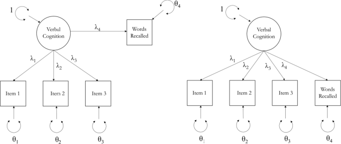
Illustration of interpretation confounding when using a simultaneous approach. The path diagram on the left shows Words Recalled intended as outcome, the path diagram on the right shows Words Recalled intended as an indicator variable. These two models are mathematically indistinguishable despite theoretical differences between them

Though multistage approaches contain more sources of error because they pass scores across stages, Devlieger et al. (2016) have shown that the performance of a multistage approach with corrections to parameter estimates and standard errors very closely approximate the performance of the simultaneous approach. Multistage approaches possess the added benefit that the measurement model is estimated in a separate first stage, meaning that misspecifications do not permeate across different parts of the model (Hayes & Usami, 2020b) and that estimation is more stable with smaller sample sizes (Rosseel, 2020). The multistage approach has recently been extended to fit measures (Devlieger et al., 2019), path analysis (Devlieger & Rosseel, 2017), and multilevel settings (Devlieger & Rosseel, 2019), giving advantages to multistage approaches broader coverage and narrowing the gap between their performance and the performance of the simultaneous approach.

For this reason, Hayes and Usami (2020a) note that the pendulum of best practice has recently swung back towards favoring multistage approaches (p. 6), but methodological debates about how to best use scores from latent variables in subsequent analyses. The important point here is that although factor scores are proxies of the true latent score, sum scores are a naïve proxy for factor scores from heavily constrained models – they are a proxy of a proxy. So, although there are still lingering questions about the best approach for using scores in subsequent analyses (i.e., a multistage approach with corrections vs. a simultaneous approach), the answer to these questions will definitively not be “sum scores”.

The next section provides an example to demonstrate how the choice of scoring method can affect conclusions when the point of obtaining scores is to use them in a subsequent analysis.

How scoring approaches can change conclusions

The Holzinger and Swineford (1939) data contained students who attended two different schools: 145 students attend the Grant-White school (48%) and 156 students attended the Pasteur school (52%). Imagine that the motivation for scoring the six cognitive items was to assess the question that there were differences in scores between these schools. The ultimate model of interest is a general linear model: the scale score(s) are the outcome and School Membership is the grouping variable (i.e., a two-group test).

We will treat the scoring of the six cognitive items in four different ways to represent different levels of rigor in order to show how the conclusions could change. Because some methods yield multiple subscales, we estimate models with a structural equation model using robust maximum likelihood estimation to fit both outcomes into a single multivariate regression model. The four methods we use are listed below. The factor score regression method with Croon’s correction in Method 3 has a dedicated function in lavaan and is easier to perform than in Mplus, so we perform all analyses in lavaan for consistency.

• 1. First, we treat the scale as if it were a researcher-created scale by which the common “alpha-and-sum” approach was applied and for which evidence of internal structure is rarely assessed (e.g., Flake et al., 2017). As noted earlier, coefficient alpha of all six cognition items together is 0.72 which is above the traditional 0.70 cut-off and the items are consequently summed to create a single score. This single score is used as the outcome in a univariate general linear model with School Membership as the predictor.

• 2. Second, the next level of rigor is to perform basic psychometric modeling to assess the internal structure but then sum score each subscale. As noted earlier, the two-factor model in Fig. 6 fit well and contained a Verbal Cognition subscale and a Speeded Cognition subscale. Sum scores are created for each subscale and are then used as observed outcomes in a multivariate general linear model with School Membership as a predictor.

• 3. Third, we use the same two-factor model from Fig. 6 but apply a multistage factor score regression. In the first stage, we Bartlett score the subscales because the latent variables are the outcome of interest, in accordance with recommendations from Skrondal and Laake (2001). Then, we apply Croon’s correction to these factor scores and use the factor scores as observed outcomes in a multivariate general linear model with School Membership as a predictor in the second-stage model.

• 4. Fourth, we use a simultaneous approach to fit the multivariate general linear with School Membership as a predictor and the latent variables from the two-factor model in Fig. 6 directly as the outcome variable such that no tangible scores are produced. This combines the measurement model and the general linear model into one large model.

Results

Here, we report the coefficients for the School Membership difference across methods. Because sum scores and factor scores are on different scales, we report both the unstandardized coefficient (B) and Cohen’s d for each effect. The first method of summing all six items yields a significant effect of School Membership (B = .99, d = .22, p = .05 ) with the conclusion that Pasteur scored higher than Grant-White (Pasteur is coded as 1 in the data, so positive coefficients indicate better performance in Pasteur). With the second method of sum scoring each subscale, the result is that Pasteur scored higher on the Verbal Cognition subscale (B = 1.68, d = .52, p < .01) but Grant-White scored higher on the Speeded Cognition subscale (B =  − .69, d =  − .28, p = .02). The third method used Croon-corrected Bartlett factor scores in a multistage factor score regression and yielded the result that Pasteur scored higher on Verbal Cognition (B = .54, d = .56, p < .01) and that there was no difference on Speeded Cognition (B =  − .17, d =  − .26, p = .07). Lastly, the fourth method is the simultaneous approach that directly uses the latent variable in the model and yielded the same result as the third method such that Pasteur scored higher on Verbal Cognition (B = .54, d = .56, p < .01) and that there was no significant difference on Speeded Cognition (B =  − .25, d =  − .34, p = .09).

Notably, sum scoring gives different conclusions compared to more rigorous methods that have been shown in the methodological literature to provide more accurate estimates. Sum scoring leads to a conclusion that Pasteur scores higher in general or that there is a dichotomy whereby Pasteur is significantly higher on Verbal Cognition and Grant-White is significantly higher on Speeded Cognition. Factor score regression and the simultaneous approach both indicate that Pasteur is higher on Verbal Cognition and there is no difference on Speeded Cognition. Essentially, the test result changes both in direction and significance depending on how the scale is scored. Furthermore, note that these different conclusions regarding Speeded Cognition between sum scores and more rigorous approaches was observed even though the correlation between Speeded Cognition sum scores and Bartlett factor scores was 0.985. At this correlation, the R² between sum scores and factor scores is 0.970, but the 3% of the variability between different scoring methods that is attributable to extraneous factors is sufficient to change the conclusion between scoring methods.

Moreover, even with a simple model that boils down to a multivariate two-group test, the ultimate inferential conclusions could change strictly based on the scoring method. The statistical models that are used in empirical studies are often vastly more complex, so results from multilevel models, growth models, or multiple regression based on sum scores may be more adversely affected by imprecision when scoring of multiple scales is necessary. Statistical methodology continues to develop at a rapid pace with methods like network models, growth mixture models, and machine learning becoming more mainstream. However, despite the exciting new research questions that can be addressed with these methods, fidelity of conclusions from these methods remains restricted by the quality of the scales and the variables analyzed from them. As one recent example, Jacobucci and Grimm (2020) note how the effectiveness of machine learning algorithms is vastly reduced in the face of imprecise measurement. This work aligns with our thesis – regardless of model complexity, the variable remains the foundational unit to which these methods are applied and complex methodology cannot solve fundamental issues associated with imprecise measures that researchers often overlook or ignore.

Discussion and limitations

Given the nature of the topics under investigation in psychology, many research studies rely on multiple-item scales to tap constructs that are not directly measurable with physical instruments. These constructs are typically complex, contextual, and multi-dimensional, rendering psychological measurement inherently more challenging than physical measurement (Michell, 2012). Variables created from scoring these scales often play a central role in subsequent analyses, either as predictor variables or as the outcome of interest. However, when justification for the scoring of scales is relegated to secondary status as is often the case when sum scores are created, it can lead to hidden ambiguity in research conclusions about the intrinsic meaning represented by the variable.

The scores from multiple-item scales are treated seriously by producers and consumers of research but the process by which those scores are obtained often is not. There are countless modeling decisions that one can make that lead to the creation of these scores – are the items treated as continuous or discrete? Do any response categories need to be collapsed or reverse coded? Are there subscales present in the scale? Whenever responses from multiple items are combined by some method, there is a model corresponding to that method. Although summing item responses may seem like a simple arithmetic operation, it is a simple linear transformation of a heavily constrained parallel factor model. Treating the sum scoring as a psychometric model rather than an arithmetic calculation obliges researchers to engage with model constraints they are imposing (perhaps unknowingly) and test the assumptions associated with such constraints.

Our point is that any method advanced by researchers for scoring scales needs evidence to support its use, and considering sum scores as a factor model demands such evidence. Neither the physical nor social sciences would endorse conclusions without evidence, so why does psychology so readily accept conclusions derived from analyses based on sum scores created without any accompanying evidence? Such v-hacking and v-ignorance (where v is shorthand for validity; Hussey & Hughes, 2019) may be contributors of replication and measurement issues in psychology; if scales are scored using untested psychometric models with unknown or questionable properties, it is difficult to replicate findings or infer meaning.

Our main point is that any scoring method corresponds to a model and any choice should be accompanied by evidence. Sum scoring is not a particularly complex model, but it is still a model nonetheless and it is possible that its assumptions could be satisfied. Several types of evidence need to be reported to support that decision: Is there sufficient unidimensionality of the scale or of each subscale? Is the internal structure supported? Are loadings sufficiently similar such that each of the items contribute about equally to what is being measured? Are there changes in reliability of the scores with different scoring methods? Perhaps there are some instances where sum scores are justified; the problem permeating throughout psychology is employing methods without any justification. We implore researchers to take psychometrics as seriously as other statistical procedures and provide justification for whichever scoring method they choose. After all, variables are the foundational unit of any statistical analyses: if the variables are not trustworthy or do not represent the constructs as intended, any results are dead-on-arrival as other modeling choices are ill-equipped to overcome deficiencies in the meaning of the variables.

Limitations

Model fit assessment

Cut-offs for model fit measures for factor models are imprecise and are used pragmatically rather than dogmatically. The commonly referenced Hu and Bentler (1999) cut-offs are based on empirical simulation rather than analytic derivation and therefore are limited by the conditions included in the simulation design. Several studies have noted that the cut-offs for many popular indices – including CFI, RMSEA, and SRMR that we use in this paper – vary with the size of the loadings (Hancock & Mueller, 2011; McNeish, An, & Hancock, 2018), size of error variances (Heene, Hilbert, Draxler, Ziegler, & Buhner, 2011), model type (Fan & Sivo, 2005), model size (Shi, Lee, & Terry, 2018), degree of misspecification (Marsh, Hau, & Wen, 2004), and missing data percentage (Fitzgerald, Estabrook, Martin, Brandmaier, & von Oertzen, 2018). We openly acknowledge the lack of firm recommendations on how to adjudicate what constitutes a “good” fitting model, but ultimately believe that imprecise metrics are an improvement over no metrics at all.

Multiple types of validity

In our examples, we focus upon one common type of evidence of validity evidence (i.e., internal structure) and one quantitative method that could be used to provide such evidence (i.e., factor analysis). The Standards for Educational and Psychological Assessment name five types of evidence, none of which are inherently more important than the other. There is an extensive literature on the theory of measurement itself; for example, Maul (2017) demonstrates that good fitting models are not inherently evidence of good theory; Borsboom, Mellenbergh, & van Heerden (2004) discredit the nomological network and argue that validity is simply the causal relationship between variation in the attribute and variation in the response; while Michell (2012) argues that measurement is not possible in the social sciences as social scientists have not established evidence of quantitivity in the attributes they claim to measure. For this reason, we focused on classic, widely reported quantitative methods such as coefficient alpha and factor analysis. Variables are the foundation of any statistical analysis, and methodological principles devised to combat data analytic issues are irrelevant if the foundational unit to which they are applied is questionably reflective of the intended construct. We offer this paper as a starting point to hopefully bridge readers from reflexively sum scoring to the more nuanced literature on scales and psychological measurement.

Take-home points

• 1. Sum scoring falls under the same umbrella as factor analysis, though it is rarely presented as such. Researchers need to be more diligent in providing support for sum scores (or an alternative scoring method), as they would with any other type of statistical model.

• 2. Considering sum scores as a latent variable model encourages researchers to evaluate the psychometric properties of their scale.

• 3. If using a previously validated scale, researchers need to verify how the scale was validated (e.g., the dimensionality of the scale). If a congeneric model was used for validation, sum scoring will apply a different unvalidated scoring model.

• 4. When using scores in subsequent analyses, the choice of scoring method can affect the conclusions of the analysis, even when the correlation between sum scores and factor scores is very high.

• 5. There are multiple methods to calculate factor scores: Bartlett scores are suggested when the score will be used as an outcome, MAP scores are suggested when the score will be used as a predictor. If saving factor scores for use in a subsequent model, researchers should be aware of possible corrections such as Croon’s correction needed to yield unbiased estimates.

• 6. Researchers can avoid decisions about different factor scoring by using a simultaneous approach that imbeds a measurement model within a broader structural equation model. This approach is considered more pure than multistage approaches, but it can result in estimation difficulties, especially with large models or small samples. In these cases, multistage approaches show similar performance with reduced estimation difficulties. Nonetheless, the distinction between multistage and simultaneous approaches is much finer than the distinction between either method and sum scoring.

Appendix

Specifying a model to obtain factor scores that exactly equal sum scores

In the main text, we show how scores from a parallel model are perfectly related to the sum scores. However, to make this equivalence more concrete, some readers may wish to know how to specify the model so that latent variable scores are exactly equal to the sum scores. Rose, Wagner, Mayer, and Nagengast (2019) formally showed how this can be accomplished and we demonstrate their method with the example six-item cognitive ability score.

In general, one variable is arbitrarily selected as a referent item. The loading from the latent variable to the referent item is then fixed to 1. The referent indicator is then regressed on all other items with all coefficients constrained to – 1. All non-referent indicators freely covary with each other and freely covary with the latent variable. The means of all non-referent items are also estimated, as is the variance of the latent variable. Figure 11 shows the path diagram for the example six item cognitive ability scale using item 6 as the referent item; the freely estimated covariances between each non-referent item and the latent variable are not shown in order to keep the path diagram as interpretable as possible.

We fit this model in Mplus version 8.2 with maximum likelihood estimation and saved the factor scores from the model. These scores are plotted against the sum scores in Fig. 12, showing that two scores remain a perfect linear transformation but now the transformation is an identify function such that the sum scores are equal to one times the factor scores and vice versa.

If using this model, Rose et al. (2019) note that fit indices cannot be calculated in traditional ways because of the non-nestedness of the standard null model in most software and the fact that variances and covariance of scale items are unrestricted. Rose et al. (2019) discuss proper calculation of fit as well as issues related to missing data.

Fig. 11

Path diagram of model to yield factor scores that perfectly correspond to sum scores. Not shown are the freely estimated covariances between all non-referent items on the left and the latent variable on the right

Fig. 12

Plot of scores from model in Fig. 11 with sum scores. The scores remain a perfect linear transformation and the transformation is now an identity function such that the two scores are equal

References

Armor, D. J. (1973). Theta reliability and factor scaling. Sociological Methodology, 5, 17–50.
American Educational Research Association, American Psychological Association, & National Council on Measurement in Education. (2014). Standards for Educational and Psychological Testing. Washington, D.C.: American Psychological Association.
Bagby, R. M., Ryder, A. G., Schuller, D. R., & Marshall, M. B. (2004). The Hamilton depression rating scale: Has the gold standard become a lead weight? The American Journal of Psychiatry, 161, 2163–2177.
Bagozzi, R. P., & Yi, Y. (1989). On the use of structural equation models in experimental designs. Journal of Marketing Research, 26, 271–284.
Barrett, P. (2007). Structural equation modelling: Adjudging model fit. Personality and Individual Differences, 42, 815–824.
Barry, A. E., Chaney, B., Piazza-Gardner, A. K., & Chavarria, E. A. (2014). Validity and reliability reporting practices in the field of health education and behavior. Health Education & Behavior, 41, 12–18.
Bartlett, M. S. (1937). The statistical conception of mental factors. British Journal of Psychology, 28, 97–104.
Bauer, D.J. & Curran, P.J. (2015). The discrepancy between measurement and modeling in longitudinal data analysis. In J.R. Harring, L.M. Stapleton & S.N. Beretvas (Eds.), Advances in Multilevel Modeling for Educational Research (pp. 3–38). Information Age Publishing.
Beck, A. T., Steer, R. A., & Garbin, M. G. (1988). Psychometric properties of the beck depression inventory: Twenty-five years of evaluation. Clinical Psychology Review, 8, 77–100.
Beck, A.T., Steer, R.A., & Brown, G.K. (1996). Manual for the Beck Depression Inventory-II. San Antonio, TX: Psychological Corporation.
Blevins, C. A., Weathers, F. W., Davis, M. T., Witte, T. K., & Domino, J. L. (2015). The posttraumatic stress disorder checklist for DSM-5 (PCL-5): Development and initial psychometric evaluation. Journal of Traumatic Stress, 28, 489–498.
Bollen, K., & Lennox, R. (1991). Conventional wisdom on measurement: A structural equation perspective. Psychological Bulletin, 110, 305–314.
Bollen, K. A. (1989). Structural equations with latent variables. New York: Wiley.
Bollen, K. A. (2002). Latent variables in psychology and the social sciences. Annual Review of Psychology, 53, 605–634.
Bollen, K. A. (2007). Interpretational confounding is due to misspecification, not to type of indicator: Comment on Howell, Breivik, and Wilcox (2007). Psychological Methods, 12, 219–228
Borsboom, D., Mellenbergh, G. J., & Van Heerden, J. (2003). The theoretical status of latent variables. Psychological Review, 110, 203–219.
Borsboom, D., Mellenbergh, G. J., & van Heerden, J. (2004). The concept of validity. Psychological Review, 111, 1061–1071.
Braun, H. I., & Mislevy, R. (2005). Intuitive test theory. Phi Delta Kappan, 86, 488–497.
Brown, T. A. (2006). Confirmatory factor analysis for applied research. New York, NY: Guilford Press.
Brydges, C. R., Reid, C. L., Fox, A. M., & Anderson, M. (2012). A unitary executive function predicts intelligence in children. Intelligence, 40, 458–469.
Burt, R. S. (1976). Interpretational confounding of unobserved variables in structural equation modeling. Sociological Methods & Research, 5, 3–53.
Cattell, R. B. (1973). Cattell Culture Fair Intelligence Test. Champaign, IL: Institute for Personality and Ability Testing
Corbisiero, S., Mörstedt, B., Bitto, H., & Stieglitz, R-H. (2017). Emotional dysregulation in adults with attention-deficit/hyperactivity disorder: Validity, predictability, severity, and comorbidity. Journal of Clinical Psychology, 73, 99–112.
Croon, M. (2002). Using predicted latent scores in general latent structure models. In G. Marcoulides & I. Moustaki (Eds.), Latent variable and latent structure modeling (pp. 195– 223). Mahwah, NJ: Lawrence Erlbaum
Crutzen, R., & Peters, G. J. Y. (2017). Scale quality: alpha is an inadequate estimate and factor-analytic evidence is needed first of all. Health Psychology Review, 11, 242–247.
Devlieger, I., & Rosseel, Y. (2017). Factor score path analysis. Methodology, 13, 31–38.
Devlieger, I., Mayer, A., & Rosseel, Y. (2016). Hypothesis testing using factor score regression: A comparison of four methods. Educational and Psychological Measurement, 76, 741–770.
Devlieger, I., Talloen, W., & Rosseel, Y. (2019). New developments in factor score regression: fit indices and a model comparison test. Educational and Psychological Measurement. Advance online publication.
Dima, A. L. (2018). Scale validation in applied health research: Tutorial for a 6-step R-based psychometrics protocol. Health Psychology and Behavioral Medicine, 6, 136–161.
diSessa, A. (1983). Phenomenology and the evolution of intuition. In D. Gentner and A. Stevens (Eds.), Mental models. (pp. 15–33) Hillsdale, NJ: Erlbaum.
DiStefano, C., Zhu, M., & Mindrila, D. (2009). Understanding and using factor scores: Considerations for the applied researcher. Practical Assessment, Research & Evaluation, 14, 1–11.
Dunn, T. J., Baguley, T., & Brunsden, V. (2014). From alpha to omega: A practical solution to the pervasive problem of internal consistency estimation. British Journal of Psychology, 105, 399–412.
Edwards, J. R., & Bagozzi, R. P. (2000). On the nature and direction of relationships between constructs and measures. Psychological Methods, 5, 155–174.
Fan, X., & Sivo, S. A. (2005). Sensitivity of fit indexes to misspecified structural or measurement model components: Rationale of two-index strategy revisited. Structural Equation Modeling, 12, 343–367.
Fava, J. L., & Velicer, W. F. (1992). An empirical comparison of factor, image, component, and scale scores. Multivariate Behavioral Research, 27, 301–322.
Fitzgerald, C. E., Estabrook, R., Martin, D. P., Brandmaier, A. M., & von Oertzen, T. (2018). Correcting the bias of the root mean squared error of approximation under missing data. https://doi.org/10.31234/osf.io/8etxa
Flake, J. K., & Fried, E. I. (2019). Measurement schmeasurement: Questionable measurement practices and how to avoid them. PsyArxiv preprint, https://doi.org/10.31234/osf.io/hs7wm
Flake, J. K., Pek, J., & Hehman, E. (2017). Construct validation in social and personality research: Current practice and recommendations. Social Psychological and Personality Science, 8, 370–378.
Fried, E. I., & Flake, J. K. (2018). Measurement matters. APS Observer, 31.
Fried, E. I., & Nesse, R. M. (2015). Depression sum-scores don’t add up: Why analyzing specific depression symptoms is essential. BMC Medicine, 13, 1–11.
Furr, M. (2011). Scale construction and psychometrics for social and personality psychology. London: Sage.
Gerbing, D. W., & Anderson, J. C. (1988). An updated paradigm for scale development incorporating unidimensionality and its assessment. Journal of Marketing Research, 25, 186–192.
Goldberg, L. W., & Digman, J. M. (1994). Revealing structure in the data: Principles of exploratory factor analysis. In S. Strack & M. Lorr (Eds.), Differentiating normal and abnormal personality (pp. 216—242). New York: Springer.
Graham, J. M. (2006). Congeneric and (essentially) tau-equivalent estimates of score reliability: What they are and how to use them. Educational and Psychological Measurement, 66, 930–944.
Graham, J. M. (2008). The general linear model as structural equation modeling. Journal of Educational and Behavioral Statistics, 33 485–506.
Green, S. B., & Yang, Y. (2009). Commentary on coefficient alpha: A cautionary tale. Psychometrika, 74, 121–135.
Green, S. B, Lissitz, R. W., & Mulaik, S. A. (1977). Limitations of coefficient alpha as an index of test unidimensionality. Educational and Psychological Measurement, 37, 827–838.
Grice, J. W. (2001). Computing and evaluating factor scores. Psychological Methods, 6, 430–450.
Hancock, G. R. & Mueller, R. O. (2001). Rethinking construct reliability within latent variable systems. In R. Cudeck, S. du Toit, & D. Sorbom (Eds.) Structural equation modeling: Present and future—A Festschrift in honor of Karl Joreskog, (pp. 195–216). Lincolnwood, IL: Scientific Software International.
Hancock, G. R., & Mueller, R. O. (2011). The reliability paradox in assessing structural relations within covariance structure models. Educational and Psychological Measurement, 71, 306–324.
Hayes, T., & Usami, S. (2020a). Factor score regression in the presence of correlated unique factors. Educational and Psychological Measurement, 80, 5–40.
Hayes, T., & Usami, S. (2020b). Factor Score Regression in Connected Measurement Models Containing Cross-Loadings. Structural Equation Modeling, advance online publication.
Heene, M., Hilbert, S., Draxler, C., Ziegler, M., & Bühner, M. (2011). Masking misfit in confirmatory factor analysis by increasing unique variances: A cautionary note on the usefulness of cutoff values of fit indices. Psychological Methods, 16, 319–336.
Hogan, T. P., Benjamin, A., & Brezinski, K. L. (2000). Reliability methods: A note on the frequency of use of various types. Educational and Psychological Measurement, 60, 523–531.
Holzinger, K. J., & Swineford, F. A. (1939). A study of factor analysis: The stability of a bi-factor solution (No. 48). Chicago: University of Chicago Press.
Hoshino, T., & Bentler, P. M. (2013). Bias in factor score regression and a simple solution. In A. R. de Leon & K. C. Chough (Eds.), Analysis of mixed data: Methods & applications (pp. 43–61). Boca Raton, FL: Chapman & Hall.
Hu, L. T., & Bentler, P. M. (1999). Cutoff criteria for fit indexes in covariance structure analysis: Conventional criteria versus new alternatives. Structural Equation Modeling, 6, 1–55.
Hussey, I., & Hughes, S. (2019). Hidden invalidity among fifteen commonly used measures in social and personality psychology. Advances in Methods and Practices in Psychological Science, advance online publication.
Jacobucci, R., & Grimm, K. (2020). Machine learning and psychological research: The unexplored effect of measurement. Perspectives on Psychological Science, advance online publication.
Joreskog, K. G. & Sorbom, D.(1979). Advances in factor analysis and structural equation models. Cambridge, MA: Abt Books.
Levy, R. (2017). Distinguishing outcomes from indicators via Bayesian modeling. Psychological Methods, 22, 632–648.
Lu, I. R., & Thomas, D. R. (2008). Avoiding and correcting bias in score-based latent variable regression with discrete manifest items. Structural Equation Modeling, 15, 462–490.
Marsh, H. W., Hau, K. T., & Wen, Z. (2004). In search of golden rules: Comment on hypothesis-testing approaches to setting cutoff values for fit indexes and dangers in overgeneralizing Hu and Bentler's (1999) findings. Structural Equation Modeling, 11, 320–341.
Matsunaga, M. (2010). How to factor-analyze your data right: Do's, don'ts, and how-to's. International Journal of Psychological Research, 3, 97–110.
Maul, A. (2017). Rethinking traditional methods of survey validation. Measurement: Interdisciplinary Research and Perspectives, 15, 51–69.
McNeish, D. (2018). Thanks coefficient alpha, we’ll take it from here. Psychological Methods, 23, 412–433.
McNeish, D., An, J., & Hancock, G. R. (2018). The thorny relation between measurement quality and fit index cutoffs in latent variable models. Journal of Personality Assessment, 100, 43–52.
Michell, J. (2012). Alfred Binet and the concept of heterogeneous orders. Frontiers in Psychology, 3, 1–8.
Millsap, R. E. (2007). Structural equation modeling made difficult. Personality and Individual Differences, 42, 875–881.
Moller, S. , Apputhurai, P., & Knowles, S. R. (2019). Confirmatory factor analyses of the ORTO 15-, 11- and 9-item scales and recommendations for suggested cut-off scores. Eating and Weight Disorders - Studies on Anorexia, Bulimia and Obesity, 24, 21–28.
Mulaik, S. (2007). There is a place for approximate fit in structural equation modelling. Personality and Individual Differences, 42, 883–891.
Peters, G. J. Y. (2014). The alpha and the omega of scale reliability and validity: why and how to abandon Cronbach’s alpha and the route towards more comprehensive assessment of scale quality. European Health Psychologist, 16, 56–69.
Reise, S. P., Waller, N. G., & Comrey, A. L. (2000). Factor analysis and scale revision. Psychological Assessment, 12, 287–297.
Revelle, W., & Zinbarg, R. E. (2009). Coefficients alpha, beta, omega, and the glb: Comments on Sijtsma. Psychometrika, 74, 145.
Rose, N., Wagner, W., Mayer, A., & Nagengast, B. (2019). Model-based manifest and latent composite scores in structural equation models. Collabra: Psychology, 5, 9.
Rosseel, Y. (2012). Lavaan: An R package for structural equation modeling. Journal of Statistical Software, 48, 1–36.
Rosseel, Y. (2020). Small sample solutions for structural equation modeling. In R. Van de Schoot & M. Miočević (Eds.), Small sample size solutions: A guide for applied researchers and practitioners (pp. 226–238). New York: Routledge.
Satnor, D. A., Gregus, M., & Welch, A. (2009). Eight decades of measurement in depression. Measurement, 4, 135–155.
Schmitt, N. (1996). Uses and abuses of coefficient alpha. Psychological Assessment, 8, 350–353.
Sharpe, D. (2013). Why the resistance to statistical innovations? Bridging the communication gap. Psychological Methods, 18, 572–582.
Shi, D., Lee, T., & Terry, R. A. (2018). Revisiting the model size effect in structural equation modeling. Structural Equation Modeling, 25, 21–40.
Skrondal, A., & Laake, P. (2001). Regression among factor scores. Psychometrika, 66, 563–575.
Steegen, S., Tuerlinckx, F., Gelman, A., & Vanpaemel, W. (2016). Increasing transparency through a multiverse analysis. Perspectives on Psychological Science, 11, 702–712.
Steiger, J. H., & Schönemann, P. H. (1978). A history of factor indeterminacy. In S. Shye (Ed.), Theory construction and data analysis in the behavioral sciences (pp. 136–178). San Francisco: Jossey-Bass.
Thomson, G. H. (1934). The meaning of “i” in the estimate of “g”. British Journal of Psychology, 25, 92–99.
Thomson, G. H. (1938). Methods of estimating mental factors. Nature, 141, 246.
Thurstone, L. (1935). The vectors of mind. Chicago, IL: University of Chicago Press.
Wainer, H. (1976). Estimating coefficients in linear models: It don't make no nevermind. Psychological Bulletin, 83, 213–217.
Wainer, H., & Thissen, D. (1976). Three steps towards robust regression. Psychometrika, 41, 9–34.
Weathers, F.W., Litz, B.T., Keane, T.M., Palmieri, P.A., Marx, B.P., & Schnurr, P.P. (2013). The PTSD Checklist for DSM-5 (PCL-5). Scale available from the National Center for PTSD at www.ptsd.va.gov.
Widaman, K. F. (2018). On common factor and principal component representations of data: Implications for theory and for confirmatory replications. Structural Equation Modeling, 25, 829–847.
Ziegler, M., & Hagemann, D. (2015). Testing the unidimensionality of items: Pitfalls and loopholes. European Journal of Psychological Assessment, 31, 231–237.
Zinbarg, R. E., Yovel, I., Revelle, W., & McDonald, R. P. (2006). Estimating generalizability to a latent variable common to all of a scale's indicators: A comparison of estimators for ωh. Applied Psychological Measurement, 30, 121–144.
Funding
There is no funding to report in association with this paper.
Author information
Authors and Affiliations
Contributions
Both authors jointly generated the idea for the paper. D. McNeish selected the data, analyzed the data, and created the figures. Both authors took part in writing the first draft. Both authors critically edited subsequent drafts and both authors approved of the final version for submission.
Corresponding author
Ethics declarations
Conflict of interest
The authors declare that there are no conflicts of interest with respect to the authorship of this paper.
Prior versions
A preprint of this paper has been uploaded to PsyArXiv, https://psyarxiv.com/3wy47/
Preregistration
There was no preregistration for this paper as it did not contain empirical studies.
Data, materials, & online resources
Raw data, software input files, software output files, and datasets containing output sum scores and factor scores can be found on the first author’s Open Science Framework page, located at https://osf.io/cahtb/.
Reporting
This study involved existing, publicly available data and featured no new data collection.
Ethical approval
All data are publicly available and are de-identified, so no approval is required.
Additional information
Publisher’s note
Springer Nature remains neutral with regard to jurisdictional claims in published maps and institutional affiliations.