Visual search for arbitrary objects in real scenes

Abstract

How efficient is visual search in real scenes? In searches for targets among arrays of randomly placed distractors, efficiency is often indexed by the slope of the reaction time (RT) × Set Size function. However, it may be impossible to define set size for real scenes. As an approximation, we hand-labeled 100 indoor scenes and used the number of labeled regions as a surrogate for set size. In Experiment 1, observers searched for named objects (a chair, bowl, etc.). With set size defined as the number of labeled regions, search was very efficient (~5 ms/item). When we controlled for a possible guessing strategy in Experiment 2, slopes increased somewhat (~15 ms/item), but they were much shallower than search for a random object among other distinctive objects outside of a scene setting (Exp. 3: ~40 ms/item). In Experiments 4–6, observers searched repeatedly through the same scene for different objects. Increased familiarity with scenes had modest effects on RTs, while repetition of target items had large effects (>500 ms). We propose that visual search in scenes is efficient because scene-specific forms of attentional guidance can eliminate most regions from the “functional set size” of items that could possibly be the target.

We conduct visual searches all day long: looking for milk in the refrigerator, the car keys, the exit, the parking spot, the e-mail icon, and so forth. Most of that searching is easy enough that we give it no thought as we pursue our goals. The purpose of this article is to offer some empirical insight into the apparent efficiency of search for arbitrary objects in real scenes. There is a vast literature on visual search for a target item among distracting items (for reviews, see Sanders & Donk, 1996; Wolfe 1998a, 1998b; Wolfe & Reynolds, 2008). The great bulk of this work has been done with simple stimuli, isolated on blank backgrounds (for a few examples, see Enns, 1988; Koene & Zhaoping, 2007; Olds, Graham, & Jones, 2009; Treisman, 1993). These studies have taught us a great deal about the basics of search, but there is no getting around the fact that such stimuli are highly artificial. Outside of the lab, people simply do not spend much time searching for red vertical lines, and when they do, the other items in the visual field are unlikely to be evenly divided into sets of red horizontals and green verticals. A smaller body of research has involved search for pictures of objects (e.g., Biederman, Blickle, Teitelbaum, & Klatsky, 1988; Wolfe, Horowitz, Kenner, Hyle, & Vasan, 2004; Yang & Zelinsky, 2009; with an important subset of work focused on search for face stimuli: e.g., Doi & Ueda, 2007; Hershler & Hochstein, 2005, 2006; VanRullen, 2006; Williams, Moss, Bradshaw, & Mattingley, 2005). But these studies have still involved search for isolated objects on blank backgrounds.

Natural search is conducted for objects embedded in scenes, and there have been an increasing number of studies involving real scenes. After some early work (Enoch, 1959; Kingsley, 1932), the systematic study of search in scenes began with Biederman’s experiments (Biederman, Glass, & Stacy, 1973), where he showed that coherent scene structure aids search. Wolfe (1994) used artificial aerial views to show that guidance to such basic attributes as color and orientation still operated when the targets and distractors were part of a continuous stimulus. Computational work has provided further evidence that the mechanisms of guidance, used to account for highly artificial search, could also be applied to scenes. Itti and Koch (2000, 2001) developed a model of bottom-up guidance by basic attributes that could be calculated over real scenes. Bottom-up salience, on its own, does not explain deployments of the eyes (and, presumably, of attention) over scenes (Foulsham & Underwood, 2007; Henderson, Brockmole, Castelhano, & Mack, 2007; Henderson, Malcolm, & Schandl, 2009). Subsequent work has expanded models to include top-down, user-driven guidance by basic attributes (Hamker, 2006; Navalpakkam & Itti, 2005; Zelinsky, 2008). Thus, if you know the features of what you are looking for, you can guide your attention to parts of a random display (Motter & Belky, 1998) or to a scene containing those features (Pomplun, 2006).

Other computational work has picked up on Biederman et al.’s (1973) finding that scene structure is important in search. Considerable current interest focuses on the role of scene “priors” (Droll & Eckstein, 2008; Ehinger, Hidalgo-Sotelo, Torralba, & Oliva, 2009; Hidalgo-Sotelo, Oliva, & Torralba, 2005; Torralba, Oliva, Castelhano, & Henderson, 2006) because, unlike in random displays of isolated objects, in a real scene the scene itself tells you where some objects might be found. Moreover, people appear to use this information in search. Observers know that people generally appear on horizontal surfaces (Droll & Eckstein, 2008; Torralba et al., 2006), chimneys appear on roofs (Eckstein, Drescher, & Shimozaki, 2006), and pots appear on stoves (Võ & Henderson, 2009). For a useful discussion of scene prior information in linguistic terms, see Henderson and Ferreira (2004).

The purpose of the present work is to understand why mundane search in the world is often easier than one might predict, extrapolating from what we know about search in the lab. Real scenes are complex and heterogeneous, and in principle any item in a scene might serve as the target for a search. In some experiments with real or realistic scenes, the target object changes from trial to trial (Brockmole & Henderson, 2006; Henderson et al., 2009; Hollingworth & Henderson, 2002; Malcolm & Henderson, 2009). The researchers of these studies have been interested in questions such as the nature of the search target template and the roles of bottom-up and top-down factors in these searches. Our focus is on the apparent efficiency of search in scenes. We focus on two questions: First, is search for arbitrary objects in scenes actually efficient, as assessed with experimental rather than introspective methods? Second, since we will give an affirmative answer to the first question, what guides efficient search in scenes?

Search efficiency and scenes

When discussing search for targets among distractors on homogeneous backgrounds, the standard measure of efficiency is the slope of the function relating reaction time (RT) to set size. Traditionally, search tasks that produced slopes near 0 ms/item have been called “parallel,” while those with slopes greater than about 20–25 ms/item for target-present trials have been deemed to be the products of serial search. However, the serial/parallel distinction is a theoretical claim about underlying mechanisms, and a problematic one, at that (Townsend, 1971, 1990; Townsend & Wenger, 2004). Referring to search “efficiency” has the virtue of being neutral about such issues. It simply describes the effective rate with which items can be processed in a search task (Wolfe 1998a, 1998b).

We search because we cannot fully process all items in the visual field at one time. If attentional resources are deployed at random, search is inefficient. According to Guided Search (Wolfe, 2007; Wolfe, Cave, & Franzel, 1989) and similar models, search becomes more efficient when attention can be “guided” to some subset of all of the available stimuli in the scene. Following Neider and Zelinsky (2008), we call that subset the “functional set size”—the set of items that the visual system deems worth considering as targets. In laboratory search tasks, the highest efficiencies (RT × Set Size slopes near 0 ms/item) are seen when a target is defined by a unique feature among homogeneous distractors of another sufficiently distinct feature, with the features drawn from one of the basic attributes that guide visual attention in search (Wolfe & Horowitz, 2004). Thus, red will “pop out” among green, vertical among horizontals, and so forth (Nothdurft, 1993; Treisman & Gelade, 1980). One way to describe a slope of zero is to propose that guidance has reduced the functional set size to 1, and thus search is easy, regardless of the number of distractors. As the differences between targets and distractors decrease and/or the heterogeneity of distractors increases, search efficiency declines (Duncan & Humphreys, 1989). If a target is defined by multiple features, attention can be guided to the conjunction of features, and search efficiency tends to be somewhat worse than is seen for pop-out searches (Wolfe et al., 1989). Here, the effective set size is reduced to some proportion of the full set size. For instance, if half of the items are red and the target is known to be red, the functional set size will be reduced by half, as will the slope of the RT × Set Size function.

If no basic feature information distinguishes targets and distractors, search typically proceeds at an “inefficient” rate of 20–40 ms/item for target-present trials, and a bit more than twice that for target-absent trials (Kwak, Dagenbach, & Egeth, 1991). Search becomes even more inefficient if each item takes a significant time to identify or if eye movements and fixations on each item are required. In the latter case, the rate would be dominated by the rate of voluntary eye movements: three or four saccades per second.

Search in scenes seems to be efficient, in spite of multiple properties that would seem to militate against efficiency. Distractor features (like color) tend to be heterogeneous. Objects are less clearly displayed than they would be on a homogeneous background. Targets are diverse and change from “trial” to “trial.” All of these factors would reduce search efficiency in the lab. We will argue that these factors are balanced by scene-specific forms of guidance. In addition to guidance by basic attributes such as size and color, search in scenes is guided by several varieties of “semantic” guidance, or guidance by the structure and meaning of scenes (e.g., the target-constraining effects of physics that are not found in random displays). The functional set size in real scenes is also influenced by “episodic” guidance, or guidance specific to knowledge about this particular scene. Thus, episodic guidance may influence search for your toothbrush in your bathroom, above and beyond semantic guidance, which constrains the placement of toothbrushes in bathrooms in general.

The problem of set size

Scene-specific guidance has been discussed before (e.g., Henderson & Ferreira, 2004), but not in terms of search efficiency and not with strong ties to the classic laboratory search paradigm, because of what can be called “the problem of set size.” Efficiency is defined in terms of RT × Set Size functions, and we have no satisfactory definition of set size in real scenes (Neider & Zelinsky, 2008; Rosenholtz, Li, & Nakano, 2007). Consider the scenes in Fig. 1.

Fig. 1

What are the “set sizes” in these images?

What is the set size of the image of the bedroom on the left? Is the bed one item, or are blanket and bedstead separate items? Is each pillow an item? Is a wall an item? On the right, is each tree an item—even the ones that are small and largely occluded—or is this a forest? Intuition tells us that search time must depend on the number of searchable entities in a scene and that the set of relevant entities can be changed by the search task. Thus, the line down the middle of the road might be a surface marking and not counted in the set size, unless the search task was to find a pair of curved lines.

In this study, we have adopted a brute force approach to the problem of set size. The LabelMe tool (Russell, Torralba, Murphy, & Freeman, 2008) provides a simple method for drawing polygons around regions of images and labeling them. At this writing, the LabelMe database contains over 65,000 annotated images, with over 732,508 labeled regions of varying precision. We took a set of 100 photographic images and had them exhaustively labeled so that almost every pixel in the scene was assigned to one labeled polygon. We then used the number of labeled polygons as a surrogate for set size.

For reasons like those raised above, even the seemingly simple process of exhaustively labeling scenes is fraught with difficulties. For instance, natural outdoor scenes tend to have very small numbers of labeled regions. Thus, the image on the right in Fig. 1 might be segmented into “road” and “forest,” even though it seems incorrect to consider this to be an image of set size 2. We avoided this issue by restricting ourselves to indoor scenes. We used unoccupied indoor scenes in order to sidestep the possibility that humans are somehow special items in search. We used largely domestic scenes (bedrooms, living rooms, kitchens, etc.) because our observers would be familiar with their contents, whereas this might not be true of factory floors, hospital wards, and so forth. Still, even unoccupied domestic indoor scenes present issues. Returning to Fig. 1, what do we do about the curtain and the window, two objects occupying the same place in the 2-D image? The details cannot be made out in Fig. 1, but if the picture on the wall contained images of objects, should they count as search items? What about objects seen through windows? When is each book one item, and when do they constitute a single shelf of books? Such questions may not be answerable in any general sense. Nevertheless, given a single labeler working with a relatively homogeneous class of images, we may assume that scenes containing more items will generate more labeled regions and that this brute force approach, while imperfect, will at least be positively correlated with the unknowable “true” set size. Note that the imperfections of this method are likely to lead to underestimates of the number of searchable objects, not overestimates. Thus, it is likely that set size could be reduced by labeling many books as a single item, “books.” It is much less likely that a single book would be overly labeled as “spine, lettering, pages,” and so on (though, in fact, one could search for such things).

Repeated search

In order to examine the role of episodic guidance in scenes, we need to give observers experience with scenes that could, in principle, produce episodic guidance (Võ & Wolfe, 2011). When we interact with a real scene, our real search behavior involves multiple searches over the same scene. Sitting down to a meal in a new restaurant illustrates the distinction between episodic and semantic guidance. Where is the fork? Where is the salad, the salt, your dining companion? All of these searches are constrained by semantic guidance. The fork is on the table to the left of the plate because that is where forks can be (they don’t float), and where they should be in a restaurant. The second time you search for fork or salt, there is the possibility that episodic guidance about this restaurant might come into play. There are two superficially contradictory facts about such “repeated searches.” First, it seems intuitively obvious that experience with a scene speeds search in scenes. You will find the coffee maker in your kitchen faster than a visitor will find it. Moving beyond intuition, clear evidence for detailed learning of multiple objects in a scene can be found in Hollingworth’s work (Hollingworth, 2006a, 2009; Hollingworth & Henderson, 2002). In apparent contrast, we have found that when observers search repeatedly through the same set of stimuli for hundreds of trials, search efficiency is the same at the end as it was at the beginning. Thus, if observers search through small sets of letters at a rate of about 35 ms/letter when the letters change on every trial, they turn out to search at the same 35-ms/letter rate 300 trials later (Wolfe, Klempen, & Dahlen, 2000). Of course, observers have learned the location and identity of all of the letters after 300 trials. However, in this experimental situation, accessing that memory appears to take about 100 ms/item, so it turns out to be more efficient to repeat the visual search than to use that memory (Kunar, Flusberg, & Wolfe, 2008a). The same result holds for search in scenes—in one particular case, realistic cartoon scenes, drawn with architectural rendering software (Oliva, Wolfe, & Arsenio, 2004).

How can the repeated-search results be reconciled with the obvious improvement in search with experience? Returning to Neider and Zelinsky’s (2008, 2010) concept of “functional set size,” the critical factor is that the failure to improve search efficiency with repeated search occurs only when the functional set size remains fixed in size. Thus, if you are always searching through the same, well-learned set of 6 letters, search efficiency does not improve. However, suppose that the display contains 30 letters, of which only 6 are ever queried in the search task. Initial search will be search at 35 ms/item through 30 items. As you learn that the relevant set is only these 6 items, search will transition to a much faster search through 6 items (Kunar et al., 2008a). If efficiency is calculated from the physical set size of 30, the efficiency will appear to increase. If it is calculated over the queried set size of 6, the rate will be 35 ms/item. Experience with the scene has the effect of reducing the functional set size in real scenes to the queried set size. In our earlier work on repeated search in artificial scenes (Oliva et al., 2004), observers rapidly learned to restrict search to the 3 or 6 objects in the scene that were task relevant. The rest of the objects were never targets and do not seem to have influenced search efficiency.

In the latter half of this article, we consider the situation where any object in the field can be a search target and where it is possible to have multiple searches though the same scene without repeating the search target. Referring back to Fig. 1a, we might ask, if you have searched for the curtain, the bed, and the picture, in Fig. 1a, is your search for the lamp speeded by your familiarity with the scene? We might also ask whether your second search for the picture will be influenced by the first.

We addressed questions of scene guidance and search efficiency in six experiments. In Experiment 1, observers searched for an arbitrary object in a novel scene on each trial. We found that search was highly efficient, at least as defined by the slope of the RT × Set Size function, with set size defined as the number of labeled items in a scene. The design of Experiment 1 (and, indeed, the design of the world) permitted observers to make intelligent guesses based on the typicality of the target object in the scene. (There is no point in searching for a long time for stoves in the bathroom.) In Experiment 2, we controlled for typicality and found that search for arbitrary objects becomes somewhat less efficient. However, Experiment 3 focused on search for arbitrary objects outside of a scene context, and we found search then to be much less efficient. These first three experiments point to the role of semantic guidance in the efficiency of scene search.

Experiments 4–6 allowed for the development of episodic guidance over repeated search through the same image for different targets. In these experiments, since the RT × Set Size functions were shallow, our interest was in the speeding of RT with repeated search through a scene. While there is some speeding of RT with increasing experience with a scene, there is massive speeding of RT only when observers search for a specific target for a second time. In Experiment 5, we showed that the background walls and floor need not be visible to produce the shallow RT × Set Size functions, if the objects are laid out as they would be in a complete scene. The experiment also showed that memory of the first search for a specific item in a specific location persists for hundreds of trials. In the first five experiments, word cues were used to identify the target. Experiment 6 showed that the advantage of the second search for a target is not entirely the result of learning the appearance of the specific target item on successful completion of the first search. Taken together, the last three experiments suggest that repeated search in a scene allows episodic guidance to speed search. To return to Fig. 1a, there might be 30 items in the scene, but once the target is identified as “lamp,” scene structure and observer knowledge about bedrooms provide the semantic guidance that reduces the functional set size to a fraction of the total items. With repeated search, that functional set seems to be reduced further on the second search for the same lamp. Were those hypothetical 30 items placed at random in a classic search display, search would take much longer.

Experiment 1: searching for arbitrary objects in novel scenes

Method

Stimuli

A set of 100 full-color images of indoor scenes was used. These were scenes of kitchens, living rooms, bedrooms, and so forth, such as one might find in an architectural magazine or real estate advertisement. As a result, there were no humans or animals in the scenes, and these rooms were somewhat cleaner than most occupied rooms. They were, however, “real” scenes—not scenes created in software, nor random collections of overlapping objects (Bravo & Farid, 2004). A lab employee exhaustively hand-labeled all images, drawing a polygon around each object and naming it. The names were reviewed by other lab members to reach consensus—though, as we will see, it is nearly impossible to label every object in a scene in a manner that will satisfy every viewer (“That’s not a bowl. It’s a dish.”). The number of labeled regions in each image ranged from 14 to 179 (M = 59, SD = 31, median: 53). There was a wide range of sizes of the labeled regions (area = 28 to 756,551 pixels, M = 15,023 pixels, SD = 36,624). The entire scene subtended 34 × 24 deg at an approximate viewing distance of 57.4 cm during these experiments. This restriction was not imposed during labeling.

Observers

A group of 12 observers were tested. All were paid volunteers who had given informed consent. Each had at least 20/25 visual acuity and normal color vision, as assessed by the Ishihara color blindness test.

Procedure

On each trial, a different image was presented. Before the scene appeared, a word cue was presented for 500 ms at the center of the screen. On 50% of trials, the word was drawn randomly from the names of the labeled polygons in the image for that trial. Surfaces were not allowed as targets (e.g., “wall,” “floor”), because virtually all of these scenes had visible walls, floors, and/or ceilings. On the other 50% of trials, a name of a polygon from another image was chosen as the cue word. It could only be used if the same term did not appear in the list of labeled regions for the current scene. If there were multiple instances of a term (e.g., “chair”), the probability of that term being used as the cue word increased accordingly.

After a 500-ms stimulus onset asynchrony, the scene appeared. The observers pressed one key if they believed that the cued target was present and another if it was absent. After the response, observers were given feedback on the accuracy of their response. On target-present trials, the target polygon or polygons were outlined, in green for a correct response and in red for an incorrect response. On target-absent trials, a “+” was presented at the center of the screen (green for correct responses, red for incorrect responses). Observers pressed any key to initiate the next trial, at which point the scene disappeared and the next trial began after an intertrial interval of 1,000 ms.

Because it is difficult, if not impossible, to ensure that all observers will agree on the appropriate name for a given object, observers were given the opportunity to dispute the label on any given trial. Before initiating the next trial, observers had the option of pressing the space bar if they disagreed with the labeling of the target objects. This brought up a screen with the prompt, “Please click on the box that best describes the problem,” and four blue boxes with the options “Wrong Name,” “Item Was Present,” “Item Was Absent,” “Other.” If observers selected “Other,” they were prompted to “‘Please briefly describe the error,” and then they typed in a free response describing the error.

After a brief period of instruction and practice, observers saw each of the 100 images 10 times, for 1,000 total trials. There were 10 blocks of 100 trials, with each image presented once per block in a randomized presentation order for each block.

Results

Trials with RTs less than 200 ms and greater than 5,000 ms were removed from analysis as outliers. This removed 2.4% of trials. Including these trials increased variance but did not substantially alter the patterns of data described below. Almost all of the excluded trials had long RTs. Observers disputed the labels on less than 3% of the trials (M = 29.6, SEM = 4.8). Of these 345 disputed trials, 334 were errors on which the observer reported that the requested target, deemed to be absent, was actually present (289 trials), or was absent when deemed present (45 trials). These trials were removed from the calculations of error rates and RTs.

Errors

Error rates were quite high in this experiment. Targets were missed on 17% of target-present trials, and false alarms occurred on 13% of target-absent trials. In typical laboratory search tasks in which RT is the dependent measure, miss errors tend to be less than 10%, and false alarm errors are very rare (Wolfe, Palmer, & Horowitz, 2010). Discriminability, d', was 2.09. All observers showed similar patterns of errors. Miss error rates varied from 10% to 23%, false alarms from 8% to 26%, and d' from 1.5 to 2.7. The subsequent RT analyses were performed on the correct responses.

RT data: effects of set size

Figure 2 shows average RTs as a function of set size (defined as the number of labeled regions) for the 100 images.

Fig. 2

Reaction time as a function of set size for each of the 100 images tested in Experiment 1. Each point is the average over 12 observers. Error bars indicate ±1 SEM. Green circles show correct target-present data, and pink diamonds show target-absent data. Regression lines were computed over the “main sequence” of set sizes from 25 to 85. The slopes are 5 ms/item when targets are present and 4 ms/item when they are absent

Several features of these data are worthy of comment. First, it is clear that set size, defined in these terms, is of limited use here. Standard RT × Set Size functions are monotonic and, usually, quite linear. Here, the images with the largest set sizes produced anomalously low RTs. We removed those large set sizes, and also the smallest set-size images, as outliers and computed slopes of the RT × Set Size functions for a “main sequence” from set size 25 to 85. The resulting slopes were 5 ms/item for target-present trials and 4 ms/item for target-absent trials. These were significantly greater than zero [F(1, 41) > 12, p < .001, in each case]. However, these slopes are comparable to those seen in the simplest feature searches, and it hardly seems credible to imagine that search for a bowl in a kitchen is as efficient as search for red among green. The vertical spread of points at a single set size tells us that there were significant sources of variance attributable to factors other than set size. Note that these slopes did not change significantly if the slowest trials (RT > 5,000 ms) were included.

How should we account for the pattern of RTs? Figure 3 shows four of the scenes that produced the fastest RTs.

Fig. 3

Four scenes that produce fast RTs

Clearly, these span a range of set sizes and a range of subjective clutter from quite low (Fig. 3d) to quite high (Fig. 3c). These examples also illustrate a property of real scenes that complicates the analysis of search efficiency: If you are sampling objects at random, you are going to have an easier time finding a chair in Fig. 3b than a plant, simply because there are many chairs. Could the apparent efficiency of search, shown in Fig. 2, be an artifact of the presence of multiple instances of the target item? If the goal is to be able to ask about arbitrary objects in arbitrary scenes, this is going to be a hard problem to eliminate. There are not many real scenes in which all objects are singletons. However, some objects are singletons, and it is possible to restrict analysis to trials on which the cue indicated a target that appeared only once in the scene. Figure 4 presents the results of this analysis.

Fig. 4

[COMP: Label top panel “A.” and bottom “B.”, as referred to in text.]Effects of number of targets. Panel a shows that, as the number of instances of a target increases, average RT decreases (purple circles) and hit rate increases (beige diamonds). Panel b shows average RTs binned by set size for hits (blue circles) and correct absent trials (red squares) (essentially duplicating Fig. 2). Green diamonds show singleton hits. All error bars indicate ±1 SEM

First, Fig. 4a shows that there was an effect of the number of instances of a target type. The number of instances ranged from 1 to 59 in the data set, but we restricted analysis to the range 1–6, because there were more than 200 trials in each of those cases. This range included 84% of target-present trials. In this range, there was a speed–accuracy covariance. As the number of instances went up, observers became both faster and more accurate (hit rate increases). Figure 4b plots RT × Set Size functions for the original data, here averaged over 10-item-wide bins. The critical data are the green diamonds, showing the average RTs for those trials on which the target was a singleton. Comparing average RTs for hits across bins, singleton RTs are slower [t(6) = 4.2, p = .006]; however, the slopes of the RT × Set Size functions are not different [F(1, 10) = 0.48, p = .5]. With the high error rates seen in this experiment, one should not put too much weight on the exact values of the slopes. However, the error rate for singletons did not increase markedly as the set size increased, so any speed–accuracy trade-off would have its prime effect on the intercept, raising all mean RTs. Moreover, the singletons were also more likely to have unusual or disputable labels (e.g., the singletons beginning with the letter G are “game case,” “garlic,” “glass,” “glass jar,” “glasses,” “globe,” “golden figurine,” “grandfather clock,” and “grapes.” Compare these to the most common labels: “plate,” “napkin,” “chair,” “book,” and “wine glass.”). Trials in which multiple examples of the cued target are present in the display are easier both because of the repeated instances of the same target and because these repeating objects and their names are simply more common (in the context of indoor scenes).

Effects of size and eccentricity

If set size, defined as the number of labeled regions, is a relatively poor predictor of RT, what does predict RT in search for arbitrary objects in real scenes? The effects of two rather unsurprising factors, target size and eccentricity, are illustrated in Fig. 5.

Fig. 5

[COMP: Label left panel “A.” and right “B.”]Effects of (a) target size (in pixels^–2) and (b) target eccentricity. Blue circles show data averaged over observers for all hit trials. Purple diamonds show singleton data. Larger sizes and eccentricities are not included because of insufficient data

As shown in Fig. 5a, RT drops dramatically as targets get bigger. The effect is roughly linear with the square root of the target size, quantified by the area labeled as belonging to the target. Dashed lines are the best-fit regression lines. The results for singletons are similar to the results for all data, though the RTs are somewhat longer and the effect of size is a bit greater. The largest sizes were removed from this analysis, because there were only a few observations for these large stimuli. Note that the change in mean RTs from the smallest to the largest sizes (600–800 ms) was much greater than the change in RTs for the smallest and largest set sizes (200–300 ms; Fig. 4b).

Eccentricity shows a 200- to 300-ms effect over the range of target eccentricities from 0 to 11 deg. Larger eccentricities generated too little data to be meaningfully analyzed. The odd dip in RT at medium eccentricities is probably an artifact of the presence of multiple targets. The eccentricity of “chair” in Fig. 3b, for example, would be the average eccentricity of all chairs in the given scene (also true for the size value). Since we are using an unsigned eccentricity, this will be a number greater than zero. As can be seen, the dip is not present when we look only at trials with singleton targets. Note also that this eccentricity effect appears even though eye movements are unconstrained, suggesting a bias to begin search in the middle of the image (Carrasco, Evert, Chang, & Katz, 1995; Wolfe, O’Neill, & Bennett, 1998). In these experiments, the bias was reasonable, since we cued the target identity at the center of the display. In the case of multiple targets with the same label, one could argue that it might be advisable to plot average RTs as though they were associated with the smallest eccentricity and the largest size. After all, observers are most likely to have found the largest, most central example of a multiple. In the present analysis, this seems unlikely to make much difference. The conclusion would remain that big central targets are found more rapidly than small eccentric ones.

The role of typicality

When observers are asked if object X is in scene Y, they can make an assessment of how likely it is that such an object will be in such a scene. The identity of the object is given to the observer before the search begins, and observers can quickly assess the gist of a scene when it first appears (Greene & Oliva, 2008; Oliva, 2005). Since targets on absent trials were drawn from the names of all labeled items in the set of images, the design of the experiment made it likely that a target that was present would be more typical of the scene than a target that was absent. In order to assess the role of typicality in Experiment 1, a subsidiary experiment was run in which new observers rated the typicality of 3,012 object–scene pairs. Of those pairs, 2,115 had been used in Experiment 1. Fifteen raters each rated an average of 524 pairs (min 54 pairs, max 1,302). Each pair was rated two to three times on a scale from 1 (very atypical) to 9 (very typical). The large number of pairs arose from the strategy of asking about random items in random scenes. Figure 6 shows the mean ratings as a function of trial type and set size (over the “main sequence”).

Fig. 6

Average typicality ratings as a function of set size and trial type. Error bars (±1 SEM) are generally smaller than the data point

Clearly, typicality was related to trial type. The main effect of trial type was significant by a Kruskal–Wallis test (p < .0001), and all pairwise comparisons were, likewise, significant (Dunn’s multiple comparison test, p < .0001). For present purposes, the important points are:

• 1. The target on a target-present trial was notably more typical of the scene than a randomly chosen target in a target-absent trial (as is, one supposes, true in the world).

• 2. When observers made errors, the typicality of a miss error was lower than that of a hit, and the typicality of a false alarm was higher that that of a correct absent trial.

This suggests that guessing could be a reasonable strategy, especially at the extremes of typicality. Evidence for guessing can be seen when error rate is plotted against typicality, as in Fig. 7, where miss errors rise to about over 30% at low typicality, while false alarms rise to similar levels at high typicality.

Fig. 7

Error rates as a function of typicality ratings in Experiment 1

This effect of typicality can be seen as both a “bug” and a “feature” in Experiment 1. On the one hand, it clearly indicates that the RT and slope measures shown in Figs. 2 and 4 are influenced by guessing, and one could argue that the shallow slopes are simply an artifact of typicality effects. This would be a form of speed–accuracy trade-off: If observers guess that unlikely items are absent, they will make miss errors. If they do not guess, they will have to search, and that search will take longer for larger set sizes, increasing the slope. A similar story would apply for guessing “present” for high-typicality targets. On the other hand, these results imply that intelligent use of the typicality of a target is a real part of the explanation of the efficiency of search in scenes. Real-world searches are based on an assessment of the likelihood of finding what you are looking for. Quitting rules are based on that assessment, as are judgments about ambiguous stimuli (e.g., “Is that really a pillow?” In a bedroom, yes. In the bathroom, maybe not.) Similar effects can be seen if target probability is manipulated directly (Wolfe & Van Wert, 2010).

Even if one chooses to see typicality effects as an important part of intelligent search, one would still want a version of the experiment without co-occurring typicality effects, in order to assess set-size effects in scene search. That was the purpose of Experiment 2.

Experiment 2: searching for arbitrary objects in scenes with typicality controlled

Method

Experiment 2 replicated Experiment 1, with the following changes. First, the target was present on every trial, and observers localized it with a mouse-click response. In other search experiments, we have found that this localization method produces approximately the same RT × Set Size functions as the traditional keypress (Wolfe, 2010). The localization method eliminates the value of guessing that an unusual item is absent; it will be present, and the observer needs to find it. RT was measured as the time from the appearance of the scene to the click on the presumed target. Second, we restricted the choice of scenes to those with set sizes between 20 and 80 (the “main sequence” of Exp. 1; see Fig. 2). Third, we eliminated all scene–target pairs that had been questioned by observers in Experiment 1 (though, as we will see, that did not eliminate observers’ questions). Fourth, we eliminated target items of less than 0.5 deg². This yielded 833 scene–target pairs. The average typicality rating was 7.1, with a distribution strongly skewed toward high typicality (58% rated 8 or 9). Taking set size in 10-item-wide bins, typicality varied from 6.3 to 7.8, but there was no systematic relationship of typicality and set size.

Each of the 10 observers was tested on 500 of the 833 possible trials, distributed so that each pair was seen six times across the data set. All observers were paid volunteers who had given informed consent. Each had at least 20/25 visual acuity and normal color vision, as assessed by the Ishihara test.

Results

The changes in method made Experiment 2 harder than Experiment 1. RTs were longer because it was no longer possible to quit search with an intelligent guess based on typicality and because the time to mouse-click on a target is generally longer than the time to press a key. Accordingly, in this experiment, we only discarded trials with RTs <200 and >10,000 ms. Moreover, even with our filtering of the scene–target pairs, observers still challenged some pairings. Of 142 challenges, 106 were caused by duplicated but unlabeled items. These are cases where, for example, one painting was labeled, but the observer clicked on another that was not labeled. On other trials, observers clicked outside of the region of the target object. These were deemed errors and not included in the RT analysis. With all of these sources of error or complaint removed, 84% of the trials remained. The number of trials removed from RT analysis (from all sources) was positively correlated with set size (R ² = .17, p = .004). This was driven by low error rates for the lowest set size (15–25). Over the range from 25 to 85, there was no significant correlation (R ² = .03, p = .13). The error rate was not correlated with the typicality rating (R ² = .03, p = .11).

The RT × Set Size function generated by the correct trials in Experiment 2 is shown in Fig. 8. The resulting slope is steeper than those of Experiment 1 [unpaired t test: t(20) = 4.0, p = .0007]. However, at 9.9 ms/item, it is still quite shallow. As will be seen in Experiment 3, observers are much less efficient when they must find objects outside of the scene context. A multiple regression analysis of the effects of typicality and set size revealed main effects of both factors. However, there was no interaction between the factors.

Fig. 8

The RT × Set Size function for Experiment 2. The data are averages of 10 observers. Error bars indicate ±1 SEM

Discussion

Search for arbitrary objects in real scenes in Experiment 1 was surprisingly efficient; at least, this was the case when set size was defined by the number of labeled regions in the scene. Part of that efficiency may have come from an effective guessing or quitting strategy. When an item was unlikely to be present, observers might have guessed “absent.” On the trials on which they were wrong and committed a miss error, they eliminated a hit RT. That hit RT would have been longer when the set size was bigger. Moreover, when the guess was correct, a short RT was substituted for what would have been a longer RT. Thus, if the guessing had not occurred, the slope would have been steeper, because the longest RTs were removed from the larger set sizes. In the real world, the set of items that are likely to be in a scene differs from the set of items not likely to be in the scene. Experiment 1 captured that regularity and, we may presume, allowed for guessing and/or criterion setting on that basis. Experiment 2 eliminated the advantage of guessing based on typicality, by making the targets always present and requiring observers to click on a target. This resulted in somewhat steeper slopes.

Nonetheless, the 9.9-ms/item average slope found in Experiment 2 was still relatively efficient. What was the cause of this efficiency? Were the targets and distractors simply sufficiently distinct that the target was easy to find? Or were there additional effects of guidance due to properties of the scene? In Experiment 3, we asked observers to search for a wide range of arbitrary objects in the absence of a scene context, and showed that search under these conditions was far more inefficient.

Experiment 3: searching for arbitrary objects in random displays

In Experiment 2, we wanted to assess the efficiency of search for arbitrary objects presented in more classic random-search displays, rather than in scenes. Most experiments involving search for naturalistic targets have used a restricted set of targets: for instance, teddy bears (Yang & Zelinsky, 2009); faces, cars, and houses (Hershler & Hochstein, 2005); animals and vehicles (Bravo & Farid, 2007); or food (Bravo & Farid, 2004). Even if search for arbitrary objects turns out to be efficient because different objects are represented in different parts of a high-dimensional space, one would not necessarily see this with a restricted set of stimuli. Presumably, even a diverse set of teddy bears live near each other in any object space. Some work has been done with larger sets of objects (Biederman et al., 1988; Newell, Brown, & Findlay, 2004; Wolfe et al., 2004). Perhaps the closest study to our goals is one by Vickery, King, and Jiang (2005) that featured a wide range of black-and-white naturalistic objects and yielded an inefficient average target-present slope of 42 ms/item.

Search for arbitrary objects in arbitrary scenes not only raises the issue of the diversity of search targets, but also the linked issues of clutter and crowding. Crowding and clutter would typically be thought to have negative effects on search (Bravo & Farid, 2004, 2007, 2009; Rosenholtz, Chan, & Balas, 2009; Rosenholtz et al., 2007; Vickery et al., 2005; Vlaskamp & Hooge, 2006), though the effects would vary with stimulus type (Reddy & VanRullen, 2007; Rosenholtz et al., 2009). Bravo and Farid (2004) obtained slopes of about 40 ms/item for “sparse” arrays of 6, 12, or 24 items, and 53 or 73 ms/item with crowded displays, depending on the complexity of the items. In their 2007 follow-up, study slopes were 75–100 ms/item with very crowded, overlapping objects. Even the relatively “sparse” displays of Bravo and Farid (2004) might be considered quite crowded, so in Experiment 2, we restricted displays to set sizes of 1–4 items, making it possible to have each item in a different quadrant of the field, in the uncrowded case.

Method

Stimuli

We used a diverse set of 230 full-color photographic images of objects in isolation on a white background. All objects had unique labels (i.e., just one “cupcake” or “swimming pool” in the set). Objects were not scaled by relative size. Thus, a “lollipop” and a “church door” could be about the same size. (Of course, in a 3-D world, the 2-D image of a nearby lollipop could well be the size of the 2-D image of a more distant door.) Ideally, it might have been desirable to use objects extracted from the scenes of Experiments 1 and 2. However, had we used objects cropped from the scenes, they would have varied dramatically in size. Some of the smaller items would have been all but unrecognizable out of their scene context. Moreover, many objects in the scenes were partially occluded, unlike the objects here. If simply removed from the scene, they would have appeared as object fragments. Accordingly, our choice of stimuli in this experiment might be seen as giving an advantage to the isolated objects, an advantage our observers proved unable to exploit.

Procedure

Prior to the main experiment, observers were shown all objects paired with their names. Observers were asked to verify that each object was appropriately named. In pilot work, the names had been refined to avoid obscure or ambiguous terms. Nevertheless, if the name we had assigned an object differed from the name observers would use to identify it, observers were given the option to type in an alternative name. This happened very rarely. On each trial of the main search experiment, observers saw the name of one object, chosen at random from the set of 230. Targets were present on 50% of the trials. When the target was absent, the cued name was still the name of an object in the set of 230. Target names were presented for 1,000 ms, and then the word was erased and a search array of 1, 2, 3, or 4 items appeared. Items were presented on an invisible 5 × 5 grid that subtended 18.4 deg at the 57.4-cm viewing distance. Each object fit within one of the 3.6 × 3.6 deg cells of this array. In a block of trials, items could be presented in a crowded or an uncrowded mode. In the 5 × 5 array, if the cells on the vertical and horizontal midlines are disallowed, there is a 2 × 2 array of cells in each quadrant of the field. In the crowded condition, all items were presented in the same quadrant. In the uncrowded condition, each item was in a different quadrant, in the cell farthest from fixation. Note that even the crowded condition is not very crowded. Items did not overlap. The inset in Fig. 9 shows a not-to-scale representation of a set size 4, uncrowded condition. For a crowded condition, all 4 items would be in one quadrant.

Fig. 9

Search for arbitrary objects in nonscene displays. Solid lines show best-fit regressions for correct present trials, dashed lines show correct absent trials. There is little difference between the Uncrowded (Blue lines and diamonds) and Crowded conditions (Purple lines and circles). Error bars indicate ±1 SEM. The inset is a representation, not to scale, of a set size 4, uncrowded trial

Fixation was not enforced, but, as the slopes of the RT × Set Size functions will show, the evidence is that observers did not need to or choose to fixate items before identifying them. Observers were tested in crowded and uncrowded blocks. Each block consisted of 30 practice and 300 experimental trials. Accuracy feedback was given after each trial.

Observers

A group of 10 observers were tested. All gave informed consent, had acuity of 20/25 or better, and had normal color vision as assessed by the Ishihara plates. All were paid for their time.

Results

RTs over 2,000 ms were deemed to be outliers. Two of the observers had high rates (13% and 25%) of such RTs and were removed from further analysis. For the remaining 8 observers, less than 1% of the RTs were greater than 2,000 ms. For those 8 observers, the miss error rates were 5.8% in the uncrowded condition and 4.3% in the crowded condition. This difference was statistically significant, t(7) = 3.1, p = .017. The false alarm rates were 2.2% and 2.3%, respectively, t(7) = 0.06, n.s.

Figure 9 shows the mean RT data for correct present and absent trials in crowded and uncrowded conditions.

For the present purposes, the important finding is that search for arbitrary objects in a nonscene display is inefficient. The target-present slopes of 45 and 41 ms/item are very similar to the results of Vickery et al. (2005). The main effect of set size is significant [F(3, 21) = 29.6, p < .001, η ²_p = .81]. The difference between present and absent slopes, as assessed by the interaction of target presence/absence and set size, is also significant [F(3, 21) = 3.2, p < .045, η ²_p = .31]. In this experiment, there was no evidence of a reliable difference between crowded and uncrowded displays [F(1, 7) = 0.00, p = .975, η ²_p = .00], perhaps because the “crowded” stimuli were quite distinct and fairly well separated. None of the interactions involving the crowding variable reached statistical significance.

The slopes in Experiment 3 were reliably steeper than the slopes in Experiment 2, the less efficient of the two scene search experiments [all ts(18) = 3.1, all ps < .006].

Discussion

Experiment 3 confirmed that search for arbitrary objects outside of a scene is not particularly efficient. As others have found with related methods, each additional item costs at least 40 ms. The set size range was very different from the estimated set sizes in Experiments 1 and 2. However, Vickery et al. (2005) obtained very similar slopes using set sizes of 8 and 16, so the inefficiency of search for isolated objects is not limited to very small set sizes. It would be difficult to do the present experiment with the very large set sizes of Experiments 1 and 2, because the items would either need to be small and very crowded or the field would need to be very large. In either case, it is unlikely that larger set sizes would produce small slopes in this case.

In Experiment 3, the lack of difference between the crowded and uncrowded conditions suggests that the inefficiency is not due to a need to fixate each object to eliminate crowding. If each item needed to be fixated, slopes would be much steeper, at least ~125 ms/item for target-present trials, if we assume four saccades/s and no refixations of rejected distractors. If there was a crowding effect in Experiment 3, it might be internal crowding of features within the complex objects rather than crowding between objects. Any within-object crowding effect would be the same in our “crowded” and “uncrowded” conditions.

The first three experiments showed that search in scenes is quite efficient—if efficiency is indexed by the slope of an RT × Set Size function, with set size derived from the number of labeled regions in the scene. What are the sources of that efficiency?

• 1. Experiment 3 confirmed that search for arbitrary objects is not always efficient. In classic inefficient search (e.g., search for Ts among Ls), the targets and distractors are fairly similar (e.g., all letters). Without the results of Experiment 3, it could have been proposed that classic guidance by attributes like color and size could account for the efficiency of search for an object. There are perhaps 12–18 preattentive attributes that guide search (Wolfe & Horowitz, 2004). These attributes, taken together, define a high-dimensional space. Arbitrary objects would be represented very sparsely in that space (DiCarlo & Cox, 2007). It might be very easy to discriminate between a target “cup” and other “noncup” objects. However, if that were the case, then search for arbitrary objects outside of a scene context should also have been efficient. Experiment 3, along with earlier experiments (Vickery et al., 2005), falsifies this account.

• 2. Experiment 2 showed that apparent efficiency is not just a typicality effect. In Experiment 1, typicality provided an excellent prior if one wanted to guess without bothering to search. If the target/scene pairing was rated 1 or 2 (low typicality), that target had less than a 20% chance of being present. If the rating was 8 or 9, the probability that this was a target-present trial was over 70%. In Experiment 2, however, this prior was rendered irrelevant by forcing observers to find a target every time. While the slopes increased, they remained quite efficient, significantly more efficient than the slopes for random object search in Experiment 3.

• 3. Apparent efficiency was probably not a consequence of a poor measure of set size. Set size in simple search displays is an important factor in determining the time to find a target. Experiments 1 and 2 found that number of labeled regions was a rather poor predictor of RT in scene search. It is certainly possible that the number of labeled regions in complex scenes is simply not a good stand-in for our old notion of set size. While that might be the case, it seems intuitively clear that, all else being equal, it will take longer to search through a scene containing many objects than to search through a scene with only a few objects, and it seems unlikely that the number of labeled regions was uncorrelated with the “true” set size, whatever that might be. Moreover, if the set-size measure were in error, it would likely be conservative. Parts of objects (e.g., table legs, cup handles) are potentially searchable but were not counted here. Consequently, it seems likely that any measure of set size will lead to the conclusions that observers are searching efficiently.

• 4. Structure of the scene guides search. If search for objects outside scene contexts is not efficient, while search in a scene context is efficient, it follows that the scene itself is making an important contribution to the efficiency of the search. In random displays of items, a limited set of basic features guides the deployment of attention (Wolfe & Horowitz, 2004). If you are looking for a red cup, you will not devote much attention to items of other colors. In this example, guidance by color reduces the functional set size (Neider & Zelinsky, 2008) from the set of all objects to the set of red objects. Scenes provide sources of guidance not available in random arrays of objects. Here, we will briefly describe two proposed classes of scene guidance, with the aid of Fig. 10.

  Fig. 10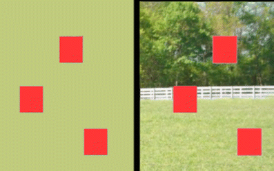

  

  Which box could just cover a horse?

Your task, in Fig. 10, is to find the box that was just covering the image of a horse. On the left side of the figure, your selection among the boxes on a blank background would be random. Not so on the right. The top box would be eliminated, because horses are generally found on surfaces that can support horses (Droll & Eckstein, 2008; Torralba et al., 2006). Borrowing language from the memory literature, we can label this constraint a form of “semantic” scene guidance. This is guidance based on generic knowledge about the world of horses, fields, and trees, as opposed to “episodic” information about this horse, this field, and this tree.

One could imagine that the top box hides a large tree house, capable of supporting an object as big as a horse. That is still not the correct box because, even if the physical constraints were met, horses do not appear in tree houses. Rather than the physics of the world, this subtype of semantic guidance is based on the regularities of specific types of scenes. Thus, we know, for example, that forks and knives often appear near plates (Bar, 2004) and chimneys appear on roofs (Eckstein et al., 2006).

The bottom box in Fig. 10 is eliminated by a third form of semantic guidance. We know something about the size of horses, and we can very rapidly assess the 3-D layout of a space (Greene & Oliva, 2009). Given these two pieces of information, the bottom box cannot hide a horse, because the horse would have to be too small to be plausible. The middle box would seem to be the best guess. Thus, various forms of semantic guidance can rapidly reduce the functional set size in a scene in ways that would not be possible in an array of random items.

As noted above, beyond generic knowledge about the world and about types of scenes, there is specific knowledge about specific scenes. There is clearly good memory for the placement of objects in scenes (Hollingworth, 2004, 2006a, 2006b, 2009), and it seems entirely reasonable to assume that you would search more efficiently for the coffee maker in your kitchen than in a novel kitchen. That said, there are limits on episodic guidance of search. In repeated search experiments in which observers searched through the same small set of letters hundreds of times, perfect knowledge of the locations of target letters did not make search more efficient (Wolfe et al., 2000), apparently because the costs of the memory search were greater than the costs of redoing the visual search (Kunar et al., 2008a). In scene search, we would expect to see effects of episodic guidance when the costs of repeating the visual search are greater than the costs of accessing the memory.

To summarize, we propose that search was more efficient in Experiments 1 and 2 because the three forms of semantic guidance could reduce the functional set size to well below the set size defined by the number of labeled regions. We know that attention and/or the eyes are guided by this sort of information (Ehinger et al., 2009; Neider & Zelinsky, 2006). The guidance based on scene information can be invoked with a very brief preview of the scene (Castelhano & Henderson, 2007; Võ & Henderson, 2010), and violations of semantic guidance impede search (Biederman, Mezzanotte, & Rabinowitz, 1982; Henderson, Weeks, & Hollingworth, 1999; Malcolm & Henderson, 2009). Many of the labeled regions simply could not be the requested target because they were the wrong size or in the wrong place. The present results tie these findings to the classic RT × Set Size measure of search efficiency.

Experiments 1–3 did not address the role of episodic guidance: When does information about the present scene guide search? That is the topic of Experiments 4–6.

Experiment 4: repeated search through the same scene

Method

In Experiment 1, the scene changed from trial to trial. In real life, it is more likely that an observer would perform a series of searches through the same scene, making the development of episodic guidance possible. In Experiment 4, observers searched 30 times through the same unchanging scene. Fifteen indoor scenes were used as stimuli, for a total of 450 trials per observer. Each scene had between 23 and 87 labeled items. For this experiment, we selected 15 items that each appeared only once in the image. The target was present on every trial, and the observers’ task was to move the mouse to click on the target. Each target item was cued twice during a block of 30 trials. The presentation order was random, so the lag between the first and second searches for a specific target could be anywhere between 1 and 29 trials.

On each trial, the mouse pointer was positioned at the center of the scene, and a word cue was presented for 500 ms below the mouse location. The scene remained visible while the cue was presented, but the mouse could not be moved until the offset of the word cue, and RT was calculated from cue offset. After the observer clicked the target location, feedback was given for 500 ms (the target polygon was outlined in green for a correct response and in red for an incorrect response). Any click within 32 pixels (1 deg) of the target polygon was counted as a correct response. After feedback was given, the mouse pointer moved back to the center of the screen, and there was a 500-ms ISI prior to the appearance of the next word cue. The scene remained continuously visible for all 30 trials.

A group of 15 observers were tested. All gave informed consent, had acuity of 20/25 or better, and had normal color vision as assessed by the Ishihara plates. All were paid for their time.

Results

Trials with RTs longer than 7,000 ms were eliminated from analysis, as were trials on which the mouse-click response fell beyond 32 pixels outside the boundary of the target object. Together, these restrictions eliminated 10% of the data.

RT × Set Size functions

Figure 11 shows the RT × set size functions for the first and second search for each target.

Fig. 11

RT × Set Size functions for the first and second searches for each target in Experiment 4. Purple circles show the first search for targets, and green diamonds show the second search. Error bars indicate ±1 SEM

As in Experiment 1, RT was only weakly related to set size, at least as defined by the number of labeled regions. Indeed, in Experiment 4, there was no significant correlation of RT and set size [first search: R ² = .12, F(1, 13) = 1.9, p = .19; second search: R ² = .04, F(1, 13) = 0.6, p = .45].

There was a highly significant difference between the first and the second search for a target [t(14) = 19.6, p < .0001]. There were two possible causes for this effect. First, observers might be faster when searching for an object that they have already found once. Second, search might become faster as the same scene is examined multiple times. The second search for an object must come after the first and, thus, the observer will have more experience with that scene. In fact, both of these factors appear to have played a role, as is shown in Fig. 12.

Fig. 12

Reaction time as a function of average position in a 30-trial block of the first (purple circles) and second (green diamonds) searches for each of the 15 targets in Experiment 4. Error bars indicate ±1 SEM

For each scene, each of the 15 targets appeared twice. Of course, the first search for the first target had to occur on the first trial. The first search for the second target could come on the second trial unless, by chance, that second trial was occupied by the second search for the first target, and so on. Figure 12 plots the RTs for each of the 15 targets as a function of the average position in the block of that target. The first repetition of the first target, for example, appears in about the sixth or seventh position, on average. The effect of experience with a particular scene can be seen in the significant declines in RTs for the first search [slope = −13.4 ms/position, R ² = .36; F(1, 13) = 7.4, p = .017] and the second search [slope = −5.6 ms/position, R ² = .49; F(1, 13) = 12.6, p = .004].

If experience with the scene were the entire cause for the improvement in RTs, then the first and second search data would lie on the same function, which they clearly do not. Experience with the specific target of search also plays a substantial role; something about the first search for the target is remembered and can be used to speed the second search for the same target (Brockmole & Henderson, 2006; C. C. Williams, 2010). The design of this experiment allowed us to examine the short-term time course of this memory. Because the two repetitions of each target were randomly placed in the block of 30 trials, the lag from first to second search varied from 1 to 29. The number of trials at each lag decreases as lag increases, but we can examine the difference between RTs for the first and second search for a target as a function of the lag between those searches. This is shown in Fig. 13.

Fig. 13

Reaction time for the first and second searches for a target in Experiment 4 as a function of the lag between those searches. Error bars indicate ±1 SEM

The robust, 600-ms difference between the first and second searches does not change as a function of lag [R ² = .006; F(1, 13) = 0.07, p = .79].

Discussion

These results suggest a two-part role for episodic guidance. To begin with, there may be a role for generalized familiarity with the scene. Returning to Fig. 12, there is a speeding of RTs over the first few searches through the scene. The regression line notwithstanding, not much improvement occurs after the first two or three trials. The more convincing effect is the large and more specific improvement seen when an object is queried for the second time. That improvement suggests that something about searching for the specific object produces strong episodic guidance. That could be memory for this object in this location or, since the cues are words, it could merely be that the observer knows what the object looks like on the second search. We will address this question in Experiment 6.

In earlier work (Wolfe et al., 2000), we found that the efficiency of repeated search through fixed displays of letters or objects did not improve, even after hundreds of searches through the same few letters. For letter search, the slope of the inferred RT × Set Size function remained quite stable at about 35–40 ms/item. In the present experiment, search appeared to be efficient at the start, and RTs improved with repetition of both scene and target. These two sets of findings are not incompatible. First, in our original repeated-search experiments, it was the slope of the RT × Set Size function that did not change; mean RTs did become faster as the task went on. Second, the failure to improve search efficiency occurs only in those cases in which all of the items in the display can be targets and are known to be potential targets. If only M of N items can be targets, search becomes apparently more efficient as observers learn to restrict their search to the relevant set of items (Kunar, Flusberg, & Wolfe, 2008b). This search might be inefficient through the relevant subset, but it can be an efficient search through the display as a whole, if the observer has learned to guide attention away from the bulk of the objects. Something of this sort may occur when observers search scenes. There might be an initial 23–89 labeled regions, but something about the scene allows the functional set size to be cut rapidly to a more manageable size. Greater exposure to the scene and to the targets in that scene makes this winnowing process more effective.

The remaining two experiments investigated the aspects of the scene that could be used to speed search.

Experiment 5: the role of the background

The scenes of Experiments 1, 2, and 4 consisted of objects and their relationships, as well as a scene “background.” In the case of our indoor scenes, the walls, floors, and so forth constituted the background. In Experiment 5, we removed that background information in order assess the contribution of the background to the efficiency of search.

Method

Experiment 5 used the same 15 scenes used in Experiment 4. In this case, however, a scene was presented in one of three conditions, illustrated in Fig. 14. An observer could see the original scene, as in Fig. 14a. In the black-background condition, only the 15 target items were presented, while the remainder of the scene was black (Fig. 14b). In the noise-background condition, the remainder of the scene was filled with a phase-scrambled, black-and-white version of the original image (Fig. 14c). Target objects retained their relative sizes and positions in the black and noise conditions. The noise condition preserved the orientation and spatial frequency content of the background as a whole but eliminated the scene structure. As can be appreciated from Fig. 14, both the black and noise conditions preserved a somewhat schematic impression of a scene.

Fig. 14

Examples of scene stimuli for Experiment 5

Each observer saw each scene twice. If a scene had one background type on its first appearance, it had the same background on the second appearance. These two appearances were generally not consecutive. More specifically, the order of scenes on first appearance was reversed on second appearance (i.e., Scenes 1, 2, 3, . . . 14, 15, followed by Scenes 15, 14, . . . 3, 2, 1). This produced a systematic variation of the lag between the first and second appearances of a scene. On each appearance of the scene, observers conducted 15 searches, 1 for each of the 15 target objects in that scene. The targets were present on every trial, and observers responded by clicking on the target. Thus, this design allowed us to look at memory for the first appearance over the longer time scale of the entire experiment, in the same way that we had looked within a 30-trial block in the previous experiment.

A group of 15 observers were tested. All had 20/25 acuity or better and had passed the Ishihara color vision test. All gave informed consent and were paid for their time.

Results

Trials were removed from the analysis if their RTs were less than 200 ms or greater than 7,000 ms, or if the observer failed to click on the target region. One observer was removed from analysis because of average RTs that were a full second longer than those of the other observers. For the remaining 14 observers, 88% of all trials were included in analysis.

As in the previous scene experiments, the effects of set size were small and often unreliable. For the black background, the RT × Set Size slope of 5.5 ms/item was statistically significant [R ² = .28; F(1, 13) = 5.1, p = .04]. For the noise background, the 5.0-ms/item slope was marginally significant [R ² = .25; F(1, 13) = 4.2, p = .06]. For the original scenes, the 2.8-ms/item slope was not significant [R ² = .09; F(1, 13) = 1.2, p = .28]. Because each observer only saw five scenes in each background condition, the power of this set-size analysis was reduced. However, if removal of the background had turned the efficient scene search of Experiment 4 into the inefficient object search of Experiment 3, the experiment would have permitted the power to detect so dramatic a change in slope.

In fact, as is shown in Fig. 15, manipulation of the background had no reliable effect on search times.

Fig. 15

Reaction time as a function of repeated search within a scene in Experiment 5. Solid symbols show the first search for a target, and open symbols show the second search. Red squares show the original scene condition, black diamonds show the black-background condition, and purple circles show the noise-background condition

As in Experiment 4, search for a target was about 600 ms faster when an observer looked for that target for a second time. Note that this second search now occurred much later than it did in Experiment 4, and other searches through other scenes had intervened. There was no clear effect of repetition within a scene. These impressions are borne out by ANOVA. The main effect of first or second search was highly statistically significant [F(1, 13) = 184.9, p < .00001, η ²_p = .93]. The effect of background was highly nonsignificant [F(2, 26) = 0.06, p = .94, η ²_p = .005], as was the effect of repetition [F(14, 182) = 0.7, p = .77, η ²_p = .07]. There was a significant interaction of background and first and second search [F(2, 26) = 6.2, p < .006, η ²_p = .32]. However, as will be discussed below, this seems to have been an artifact of imperfect counterbalancing.

Experiment 5 was designed to allow examination of memory for the first search for a target over a larger range of trials and over intervening search through other scenes. This can be seen in Fig. 16.

Fig. 16

Reaction time as a function of block in Experiment 5. Purple circles show the first 15 scenes, and green diamonds show their repetition in reverse order

Looking first at the data from the first 15 blocks, RT decreases [slope = −11.5 ms/block, R ² = .30; F(1, 13) = 5.5, p = .035], though, in fact, most of the improvement occurs over the first four blocks. Over Scenes 5–15, there is no significant change in RT [slope = −3.0 ms/block, R ² = .02; F(1, 9) = 0.2, p = .67]. Presumably, the early decrease in RT reflects the effects of training on the task, since there was nothing specific about practice with Scene 1 that should inform search through Scene 2. In contrast, the 16th block repeated the scene searched on the 15th block. There is a massive, 850-ms speeding of the search times for that block as compared to Block 15. Thereafter, RTs steadily increase [slope = 26.5 ms/block, R ² = .72; F(1, 13) = 32.7, p < .0001]. Presumably, this increase reflects the waning effects of the memory that supports the advantage for the second search for the same target in the same scene. The shorter the lag between the first and second appearances of a scene, the larger the advantage for the second search. As it happened, the lag for scenes with the original background was slightly shorter than the lag for black backgrounds, which was slightly shorter than the lag for the noise backgrounds. This failure of perfect counterbalancing appears to have been responsible for the significant Background × Appearance interaction discussed above. The interaction does not appear to show any real role for the background in guiding these searches.

Discussion

At least for this restricted set of indoor scenes, the background structure of walls, floor, and so forth does not appear to have added anything to the guidance of search. Perhaps the layout of the 15 objects allowed for adequate inference of the hidden structure in the black and noise conditions, or perhaps the critical information is in the relationships between objects: Plates are near cups. Printers and monitors rest on horizontal surfaces. Whatever is providing the information, it is clear that removing the walls, floors, and such of these indoor scenes did not weaken the semantic guidance of search within them.

Experiment 5 showed that the large advantage for the second search for a particular target in a particular scene extended to target/scene pairs that had not been seen for hundreds of trials. This episodic guidance effect is evidence for a memory reminiscent of the massive memory for objects (Brady, Konkle, Alvarez, & Oliva, 2008; Konkle, Brady, Alvarez, & Oliva, 2010) and of the impressive ability to remember the details of specific objects in specific scenes (Hollingworth 2006a, b; Hollingworth & Henderson, 2002). In Experiment 5, the episodic guidance could be seen degrading over time. Nevertheless, there was some information gathered in the first appearance of a target–scene pair that observers could remember and use to aid search, even after several hundred trials. It is worth noting that this memory seems to depend on active search for the item. If mere exposure were enough, one would expect to have seen more of an effect of the 15 repeated searches through a scene (Võ & Wolfe, 2010). In Experiment 5, there was no effect of repetition within a scene—the 15th search through the scene was no faster than the first (Fig. 15), but when 1 of the 15 targets was finally repeated, that 16th search was hundreds of milliseconds faster. The incidental examination and rejection of objects as distractors does not seem produce episodic guidance. Search for a specific item is what produces episodic guidance for the next request to find that target, unless the entire second-appearance effect was an artifact. This is the topic of the final experiment.

Experiment 6: picture cues

What was the nature of the episodic guidance that, in Experiments 4 and 5, produced very strong effects of repeating a specific target? It could be a rather unsurprising side effect of our use of word cues in all of the experiments presented so far. We know that exact picture cues produce shorter RTs in search through random arrays of objects (Castelhano & Heaven, 2010; Vickery et al., 2005; Wolfe et al., 2004). In the previous experiments, once the observer had found the target the first time, he knew what the target looked like. Perhaps the effective memory was simply the memory that the word “bowl” refers to this specific bowl, and the remembered visual attributes of this bowl could then speed search. In order to test this hypothesis, Experiment 6 replicated Experiment 4 using exact picture cues to supplement the word cue. If the effect was entirely due to the fact that observers did not know the details of the specific target on first search, then the exact picture cues should greatly reduce or eliminate the second-search advantage.

Method

As in Experiment 4, observers searched through the same scene 30 times. Each of 15 possible targets was shown twice in random order. There were 15 scenes, so each observer performed 450 trials. Targets were present on every trial, and observers clicked on the target to make a response. Critically, the target was identified on each trial by presenting its exact image, as well as its name, in the center of the scene for 1,500 ms. The long duration was required because some objects, cut from their context, were rather hard to identify. The size of the picture was jittered between 80% and 120% of the actual size so that the picture cue would not necessarily be an exact match of the target in the scene. In all other details, the design of Experiment 6 was the same as that of Experiment 4.

A group of 15 observers were tested. All had 20/25 or better acuity and had passed the Ishihara color test. All gave informed consent and were paid for their time.

Results

The primary result of Experiment 6 was that showing observers the exact search target improves performance on the first search but does not eliminate the large advantage of the second search. Removing all trials with RTs less than 200 and greater than 7,000 ms and removing all incorrect responses left 96% of the original trials. As in the other scene search experiments, the effects of set size were small and, in this case, not statistically significant. For the first search of a target item, the slope was 3.2 ms/item [R ² = .09; F(1, 13) = 1.3, p = .27], and for the second search the slope was 0.9 ms/item [R ² = .05; F(1, 13) = 0.64, p = .44].

Figure 17 shows RTs as a function of position in the 30-trial block for a scene. The equivalent data for Experiment 4, from Fig. 12, are shown in purple and green open symbols, for comparison. Recall that, because the 30 trials were presented in random order, the second search for one target could occur before the first appearance of another. Thus, on average, the first repeated target occurred on the 6th or 7th trial of the 30-trial block (the leftmost open green diamond in Fig. 17).

Fig. 17

Reaction time as a function of average position in a 30-trial block of searches through a scene. Each target appears twice. Purple circles show the first search, and green diamonds show the second search. Filled symbols show data from Experiment 6, and the open symbols reproduce the data from Experiment 4 (Fig. 12), for comparison

The main finding of Experiment 6 was that the use of picture cues reduces but does not eliminate the RT advantage for the second search for a target. The reduction comes from a speeding of the first RT. First-search RTs were faster in Experiment 6 (M = 1,449 ms) than in Experiment 4 (M = 1,813 ms), paired t(14) = 8.21, p < .001; this paired t test compared the same scenes and the same objects in the two experiments, albeit with different observers. The correlation between RTs for scenes in the two experiments was .65, R ² = .42. Second-search RTs were not significantly faster in Experiment 6 (M = 1,068 ms) than in Experiment 4 (M = 1,104 ms), paired t(14) = 1.18, p < .26. The benefit of seeing the target in advance was absent on the second search presumably because, as in the previous experiments, the word evoked a memory of the target adequate to produce the same RT.

Picture cues do not eliminate the second-search advantage [main effect of appearance: F(1, 14) = 263, p < .0001, η ²_p = .94]. In addition, there was a significant effect of repeated search through the same scene for different objects [F(14, 196) = 2.9, p = .0006, η ²_p = .16] and an interaction of first/second search and repeated-search effects [F(14, 196) = 2.9, p = .0004, η ²_p = .17]. This reflects a significant decline in RTs as a function of the number of times one has searched through a scene, for the first search of a target [−13.4 ms/repetition, R ² = .56; F(1, 13) = 16.8, p = .0013], but not when a target has already appeared once [0.3 ms/repetition, R ² = .01; F(1, 13) = 0.1, p = .76]. Note, again, that the improvement occurs over the first few trials and is absent from average Position 5 onward.

We conclude that the memory supporting the second-search advantage includes information about the relationship of the target object to the scene and not merely information about the specific features of the target.

General discussion

Why is search for arbitrary objects in indoor scenes so efficient?

The efficiency of visual search has been indexed by the slope of the function relating RT to set size. A barrier to understanding the efficiency of search in real scenes is that no one knows how to count the set size in a real scene. Our effort to use the number of labeled regions in a scene as a surrogate for set size produced very shallow RT × Set Size functions. We can reject a number of possible reasons for this apparent efficiency.

Did we overestimate the number of items in the scene?

Inflating the set size would decrease the slope. However, it seems far more likely that the number of labeled regions was an underestimate of the number of items. Aggregate labels like “books” and “pillows” make single items out of multiples, and the failure to label parts of compound objects probably eliminated searchable items like picture frames and doll dresses.

Is all search for arbitrary objects reasonably efficient?

It could be proposed that objects are sparsely represented in a high-dimensional space, with the result that it is easy for the visual system to divide that space into a region containing a given type of object, such as a “cup,” and a region containing nearly all “noncup” objects. This would be the high-dimensional equivalent of the easy search when the target is linear separable from the distractors in, for example, color space (Bauer, Jolicœur, & Cowan, 1996), and of the advantage of multidimensional feature vectors in machine classification. Experiment 3, as well as previous work reviewed earlier, showed that object search is not efficient outside of a scene context. Moreover, the efficient search for objects in scenes is still much slower than classic “pop-out” of targets defined by attributes like color, size, and so forth. Classic pop-out RTs would be on the order of 400–500 ms. These scene-search RTs asymptote at about 1,100–1,200 ms.

Did observers simply develop an effective guessing strategy?

The structure of Experiment 1 would allow for effective guessing based on the typicality of the target in the scene. If you are asked about a refrigerator in the bathroom, you can probably reply “absent” without much actual search. However, controlling for typicality in Experiment 2 produced search efficiencies that were still three to four times more efficient than search for objects in nonscene arrays.

Is the set-size estimate simply worthless?

It would be easy to get a shallow slope if the number on the x-axis were not meaningful at all. However, the count of labeled regions, flawed as it may be, does seem to be meaningfully related to the number of objects in a scene. Some scenes were problematic. If you are searching for a “chair” in a scene with 100 chairs, the set size will be over 100, but the RT required to find the first chair will be very short. However, search slopes remained shallow when data analysis was restricted to singleton targets in Experiment 1 (Fig. 4b) and when all of the targets were singletons (Exps. 4–6).

We suggest that the efficiency of these scene searches reflects an ability to use scene guidance to reduce the functional set size. Consider the kitchen scene in Fig. 3d. There may be 36 labeled items, and there would be more if individual pieces of fruit were itemized. However, if the target was “oven,” the semantic guidance would dramatically reduce the number of items that could be the target. As noted earlier, semantic guidance describes multiple types of general information about the world and about scenes of this sort (Davenport & Potter, 2004; Hollingworth & Henderson, 2000; Hwang, Wang, & Pomplun, 2011; Oliva & Torralba, 2001; Võ & Henderson, 2009). In search of an oven, semantic guidance would include the understanding that ovens need support. Thus, they do not float, and they typically sit on top of surfaces rather than hanging from the ceiling (Biederman et al., 1982). Moreover, ovens are objects of a certain size in the world. Given knowledge of the layout of the scene in Fig. 3d and the 2-D size of proto-objects in that scene, search would be limited to only a few objects that could plausibly be ovens, even without needing to identify objects or the specific scene.

The second time you are asked for the oven, episodic guidance would speed search for this oven in this scene. There is a much more modest effect on search for the oven deriving from repeated search for other objects in the same scene (Võ & Wolfe, 2011).

Scene guidance is analogous to the widely accepted concept of guided search by basic attributes like color or motion (Wolfe et al., 1989). There might be 100 letters in a display, but if you are looking for the red T, classic guidance will reduce the functional set size to the set of, say, 10 red letters (Egeth, Virzi, & Garbart, 1984). Guidance by scene information requires some analysis of the scene. However, this is not a circular proposition, where knowledge of all the objects in the scene would help you to find individual objects in the scene. There is abundant information for rapid global/parallel extraction of information about scenes without identification of the component objects. This information includes scene category (e.g., mountain, beach, urban), coarse layout (e.g., open, closed, navigable, indoor), and the presence of categories of objects (e.g., animal) (Greene & Oliva, 2008; Joubert, Rousselet, Fize, & Fabre-Thorpe, 2007; Li, VanRullen, Koch, & Perona, 2002). This sort of information contributes to the scene guidance that reduces the functional set size of search in scenes.

What is being remembered about targets in scenes?

In these experiments, the largest effects of prior exposure occurred when a specific target was searched for again in a specific scene. For this to occur, observers must have remembered the scene, the target, and the relationship of the two. It is interesting that we did not see strong evidence for the development of this sort of memory for distractor items. Incidental learning about the position of nontarget objects might account for the decline in RTs seen in the first repetitions in Figs. 12 and 17. However, the reduction in RT is much more dramatic when a target is repeated. Given the robustness of this effect, it would be interesting to examine its contents in more detail. For example, Brady et al. (2008) and Konkle et al. (2010) showed that observers are surprisingly good at remembering the pose and state of objects seen in isolation. Would we see the same massive decrease in RT on the second search for a target in the same location, but in a different pose or state (Hollingworth & Henderson, 1999)? If this were a useful memory and not a mere laboratory curiosity, one imagines that the benefit would remain. It seems unlikely that the cat needs to maintain his exact pose on the bed in order to facilitate search. On the other hand, it seems probable that a change in position in the image would disrupt the effect and that something about the nature of the spatial memory could be inferred by systematically varying the position. For instance, does the second search remain fast if the shifted target remains on the same surface?

Other types of scenes and targets

One drawback of the present set of experiments is the restricted range of scenes. The scenes were indoor domestic rooms that were without people and cleaner than average. They were also canonically posed, and one cannot rely on such a cue in real search in the real world. The bed is not always at the center of your view of a bedroom, nor is the whole table neatly visible in the middle of the image of the dining room. These images had the advantage of containing many objects that could be named by our observer population, but there is a danger that some of the results might have been specific to this class of scene. To return to an issue raised in connection with Fig. 1, search of outdoor scenes is not likely to be qualitatively different than search of indoor scenes, even though the outdoor scenes typically have many fewer labeled regions.

The use of those labeled regions as targets is a limitation of the present study. Regions were labeled with categorical, basic-level names (“glasses,” “basket,” “chest,” “coat rack,” etc.) with a few modifiers (“potted plant,” “horse statue,” “toy horse,” etc.). This procedure missed much of the specificity of description that we use intuitively to guide the search of others. Additional basic feature information is provided (“Can you see that white bird with the curved orange beak?”), as well as position relative to other objects (“It is next to the rose bush . . .”) and relative to the observer (“. . . on the left”). Once this richer form of target specification is allowed, the differences between the searchable contents of indoor and outdoor scenes will be reduced.

In summary, the results of these six experiments show that the number of labeled items in a scene is a relatively poor predictor of the amount of time that it takes to find one of those items. The scene provides information that guides search, and semantic guidance becomes available rapidly on scene onset. Episodic guidance accumulates with more experience with the scene and speeds search when the same target is searched for a second time. Support or falsification of each of these claims awaits further research with a wider range of scenes and targets.

References

Bar, M. (2004). Visual objects in context. Nature Reviews Neuroscience, 5, 617–629.
Bauer, B., Jolicœur, P., & Cowan, W. B. (1996). Visual search for colour targets that are or are not linearly-separable from distractors. Vision Research, 36, 1439–1466.
Biederman, I., Blickle, T. W., Teitelbaum, R. C., & Klatsky, G. J. (1988). Object search in nonscene displays. Journal of Experimental Psychology. Learning, Memory, and Cognition, 14, 456–467. doi:10.1037/0278-7393.14.3.456
Biederman, I., Glass, A. L., & Stacy, E. W. (1973). Searching for objects in real-world scenes. Journal of Experimental Psychology, 97, 22–27.
Biederman, I., Mezzanotte, R. J., & Rabinowitz, J. C. (1982). Scene perception: Detecting and judging objects undergoing relational violations. Cognitive Psychology, 14, 143–177.
Brady, T. F., Konkle, T., Alvarez, G. A., & Oliva, A. (2008). Visual long-term memory has a massive storage capacity for object details. Proceedings of the National Academy of Sciences, 105, 14325–14329. doi:10.1073/pnas.0803390105
Bravo, M. J., & Farid, H. (2004). Search for a category target in clutter. Perception, 33, 643–652.
Bravo, M. J., & Farid, H. (2007). The depth of distractor processing in search with clutter. Perception, 36, 812–829.
Bravo, M. J., & Farid, H. (2009). The specificity of the search template. Journal of Vision, 9(1), 34:1–9.
Brockmole, J. R., & Henderson, J. M. (2006). Using real-world scenes as contextual cues for search. Visual Cognition, 13, 99–108. doi:10.1080/13506280500165188
Carrasco, M., Evert, D. L., Chang, I., & Katz, S. M. (1995). The eccentricity effect: Target eccentricity affects performance on conjunction searches. Perception & Psychophysics, 57, 1241–1261.
Castelhano, M. S., & Heaven, C. (2010). The relative contribution of scene context and target features to visual search in scenes. Attention, Perception, & Psychophysics, 72, 1283–1297.
Castelhano, M. S., & Henderson, J. M. (2007). Initial scene representations facilitate eye movement guidance in visual search. Journal of Experimental Psychology. Human Perception and Performance, 33, 753–763.
Davenport, J. L., & Potter, M. C. (2004). Scene consistency in object and background perception. Psychological Sciences, 15, 559–564.
DiCarlo, J. J., & Cox, D. D. (2007). Untangling invariant object recognition. Trends in Cognitive Sciences, 11, 333–341.
Doi, H., & Ueda, K. (2007). Searching for a perceived stare in the crowd. Perception, 36, 773–780.
Droll, J., & Eckstein, M. (2008). Expected object position of two hundred fifty observers predicts first fixations of seventy seven separate observers during search. Journal of Vision, 8(6), 320a.
Duncan, J., & Humphreys, G. W. (1989). Visual search and stimulus similarity. Psychological Review, 96, 433–458. doi:10.1037/0033-295X.96.3.433
Eckstein, M. P., Drescher, B. A., & Shimozaki, S. S. (2006). Attentional cues in real scenes, saccadic targeting, and Bayesian priors. Psychological Science, 17, 973–980.
Egeth, H. E., Virzi, R. A., & Garbart, H. (1984). Searching for conjunctively defined targets. Journal of Experimental Psychology. Human Perception and Performance, 10, 32–39.
Ehinger, K. A., Hidalgo-Sotelo, B., Torralba, A., & Oliva, A. (2009). Modelling search for people in 900 scenes: A combined source model of eye guidance. Visual Cognition, 17, 945–978.
Enns, J. T. (1988). Three-dimensional features that pop-out in visual search. In D. Brogan (Ed.), Visual search (vol. 1) (Vol. 1). London: Taylor & Francis.
Enoch, J. M. (1959). Effect of the size of a complex display upon visual search. Journal of the Optical Society of America, 49, 280–286. doi:10.1364/JOSA.49.000280
Foulsham, T., & Underwood, G. (2007). How does the purpose of inspection influence the potency of visual salience in scene perception? Perception, 36, 1123–1138.
Greene, M. R., & Oliva, A. (2008). Recognition of natural scenes from global properties: Seeing the forest without representing the trees. Cognitive Psychology, 58, 137–176.
Greene, M. R., & Oliva, A. (2009). The briefest of glances: The time course of natural scene understanding. Psychological Science, 20, 464–472.
Hamker, F. (2006). Modeling feature-based attention as an active top-down inference process. Biosystems, 86, 91–99.
Henderson, J. M., Brockmole, J. R., Castelhano, M. S., & Mack, M. (2007). Visual saliency does not account for eye movements during visual search in real-world scenes. In R. P. G. van Gompel, M. H. Fischer, W. S. Murray, & R. L. Hill (Eds.), Eye movements: A window on mind and brain (pp. 537–562). Amsterdam: Elsevier.
Henderson, J. M., & Ferreira, F. (2004). Scene perception for psycholinguists. In J. M. Henderson & F. Ferreira (Eds.), The interface of language, vision, and action: Eye movements and the visual world (pp. 1–58). New York: Psychology Press.
Henderson, J. M., Malcolm, G. L., & Schandl, C. (2009). Searching in the dark: Cognitive relevance drives attention in real-world scenes. Psychonomic Bulletin & Review, 16, 850–856.
Henderson, J. M., Weeks, P. A., Jr., & Hollingworth, A. (1999). The effects of semantic consistency on eye movements during complex scene viewing. Journal of Experimental Psychology. Human Perception and Performance, 25, 210–228. doi:10.1037/0096-1523.25.1.210
Hershler, O., & Hochstein, S. (2005). At first sight: a high-level pop out effect for faces. Vision Research, 45, 1707–1724.
Hershler, O., & Hochstein, S. (2006). With a careful look: Still no low-level confound to face pop-out. Vision Research, 46, 3028–3035. doi:10.1016/j.visres.2006.03.023
Hidalgo-Sotelo, B., Oliva, A., & Torralba, A. (2005). Human learning of contextual priors for object search: Where does the time go? Paper presented at the 3rd International Workshop on Attention and Performance in Computer Vision, Washington, DC.
Hollingworth, A. (2004). Constructing visual representations of natural scenes: The roles of short- and long-term visual memory. Journal of Experimental Psychology. Human Perception and Performance, 30, 519–537.
Hollingworth, A. (2006a). Scene and position specificity in visual memory for objects. Journal of Experimental Psychology. Learning, Memory, and Cognition, 32, 58–69.
Hollingworth, A. (2006b). Visual memory for natural scenes: Evidence from change detection and visual search. Visual Cognition, 14, 781–807.
Hollingworth, A. (2009). Two forms of scene memory guide visual search: Memory for scene context and memory for the binding of target object to scene location. Visual Cognition, 17, 273–291.
Hollingworth, A., & Henderson, J. M. (1999). Object identification is isolated from scene semantic constraint: Evidence from object type and token discrimination. Acta Psychologica, 102, 319–343.
Hollingworth, A., & Henderson, J. M. (2000). Semantic informativeness mediates the detection of changes in natural scenes. Visual Cognition, 7, 213–235.
Hollingworth, A., & Henderson, J. M. (2002). Accurate visual memory for previously attended objects in natural scenes. Journal of Experimental Psychology. Human Perception and Performance, 28, 113–136.
Hwang, A. D., Wang, H.-C., & Pomplun, M. (2011). Semantic guidance of eye movements in real-world scenes. Vision Research, 51, 1192–1205. doi:10.1016/j.visres.2011.03.010
Itti, L., & Koch, C. (2000). A saliency-based search mechanism for overt and covert shifts of visual attention. Vision Research, 40, 1489–1506.
Itti, L., & Koch, C. (2001). Computational modelling of visual attention. Nature Reviews Neuroscience, 2, 194–203.
Joubert, O. R., Rousselet, G. A., Fize, D., & Fabre-Thorpe, M. (2007). Processing scene context: Fast categorization and object interference. Vision Research, 47, 3286–3297.
Kingsley, H. L. (1932). An experimental study of “search. The American Journal of Psychology, 44, 314–318. doi:10.2307/1414831
Koene, A. R., & Zhaoping, L. (2007). Feature-specific interactions in salience from combined feature contrasts: Evidence for a bottom-up saliency map in V1. Journal of Vision, 7(7), 6:1–14. doi:10.1167/7.7.6
Konkle, T., Brady, T. F., Alvarez, G. A., & Oliva, A. (2010). Scene memory is more detailed than you think: The role of categories in visual long-term memory. Psychological Science, 21, 1551–1556. doi:10.1177/0956797610385359
Kunar, M. A., Flusberg, S., & Wolfe, J. M. (2008a). The role of memory and restricted context in repeated visual search. Perception & Psychophysics, 70, 314–328. doi:10.3758/PP.70.2.314
Kunar, M., Flusberg, S., & Wolfe, J. (2008b). Why don’t people use memory when repeatedly searching though an over-learned visual display? Journal of Vision, 8(6), 311a.
Kwak, H., Dagenbach, D., & Egeth, H. (1991). Further evidence for a time-independent shift of the focus of attention. Perception & Psychophysics, 49, 473–480.
Li, F. F., VanRullen, R., Koch, C., & Perona, P. (2002). Rapid natural scene categorization in the near absence of attention. Proceedings of the National Academy of Sciences, 99, 9596–9601.
Malcolm, G. L., & Henderson, J. M. (2009). The effects of target template specificity on visual search in real-world scenes: Evidence from eye movements. Journal of Vision, 9(11), 8:1–13.
Motter, B. C., & Belky, E. J. (1998). The guidance of eye movements during active visual search. Vision Research, 38, 1805–1815.
Navalpakkam, V., & Itti, L. (2005). Modeling the influence of task on attention. Vision Research, 45, 205–231.
Neider, M. B., & Zelinsky, G. J. (2006). Scene context guides eye movements during visual search. Vision Research, 46, 614–621. doi:10.1016/j.visres.2005.08.025
Neider, M. B., & Zelinsky, G. J. (2008). Exploring set size effects in scenes: Identifying the objects of search. Visual Cognition, 16, 1–10. doi:10.1080/13506280701381691
Neider, M. B., & Zelinsky, G. J. (2010). Exploring the perceptual causes of search set-size effects in complex scenes. Perception, 39, 780–794. doi:10.1068/p6428
Newell, F. N., Brown, V., & Findlay, J. M. (2004). Is object search mediated by object-based or image-based representations? Spatial Vision, 17, 511–541.
Nothdurft, H.-C. (1993). The role of features in preattentive vision: Comparison of orientation, motion and color cues. Vision Research, 33, 1937–1958. doi:10.1016/0042-6989(93)90020-W
Olds, E. S., Graham, T. J., & Jones, J. A. (2009). Feature head-start: Conjunction search following progressive feature disclosure. Vision Research, 49, 1428–1447.
Oliva, A. (2005). Gist of the scene. In L. Itti, G. Rees, & J. Tsotsos (Eds.), Neurobiology of attention (pp. 251–257). San Diego: Academic.
Oliva, A., & Torralba, A. (2001). Modeling the shape of the scene: A holistic representation of the spatial envelope. International Journal of Computer Vision, 42, 145–175.
Oliva, A., Wolfe, J. M., & Arsenio, H. C. (2004). Panoramic search: The interaction of memory and vision in search through a familiar scene. Journal of Experimental Psychology. Human Perception and Performance, 30, 1132–1146.
Pomplun, M. (2006). Saccadic selectivity in complex visual search displays. Vision Research, 46, 1886–1900. doi:10.1016/j.visres.2005.12.003
Reddy, L., & VanRullen, R. (2007). Spacing affects some but not all visual searches: Implications for theories of attention and crowding. Journal of Vision, 7(2), 3:1–17.
Rosenholtz, R., Chan, S., & Balas, B. (2009). A crowded model of visual search. Journal of Vision, 9(8), 1197a.
Rosenholtz, R., Li, Y., & Nakano, L. (2007). Measuring visual clutter. Journal of Vision, 7(2), 17:1–22.
Russell, B. C., Torralba, A., Murphy, K. P., & Freeman, W. T. (2008). LabelMe: A database and web-based tool for image annotation. International Journal of Computer Vision, 77, 157–173.
Sanders, A. F., & Donk, M. (1996). Visual search. In O. Neumann & A. F. Sanders (Eds.), Handbook of perception and action: Vol. 3. Attention (pp. 43–77). London: Academic.
Torralba, A., Oliva, A., Castelhano, M. S., & Henderson, J. M. (2006). Contextual guidance of eye movements and attention in real-world scenes: The role of global features in object search. Psychological Review, 113, 766–786. doi:10.1037/0033-295X.113.4.766
Townsend, J. T. (1971). A note on the identification of parallel and serial processes. Perception & Psychophysics, 10, 161–163.
Townsend, J. T. (1990). Serial and parallel processing: Sometimes they look like Tweedledum and Tweedledee but they can (and should) be distinguished. Psychological Science, 1, 46–54.
Townsend, J. T., & Wenger, M. J. (2004). The serial–parallel dilemma: A case study in a linkage of theory and method. Psychonomic Bulletin & Review, 11, 391–418. doi:10.3758/BF03196588
Treisman, A. (1993). The perception of features and objects. In A. Baddeley & L. Weiskrantz (Eds.), Attention: Selection, awareness, and control (pp. 5–35). Oxford: Oxford University Press, Clarendon Press.
Treisman, A. M., & Gelade, G. (1980). A feature-integration theory of attention. Cognitive Psychology, 12, 97–136. doi:10.1016/0010-0285(80)90005-5
VanRullen, R. (2006). On second glance: Still no high-level pop-out effect for faces. Vision Research, 46, 3017–3027. doi:10.1016/j.visres.2005.07.009
Vickery, T. J., King, L.-W., & Jiang, Y. (2005). Setting up the target template in visual search. Journal of Vision, 5(1), 8:81–92. doi:10.1167/5.1.8
Vlaskamp, B. N. S., & Hooge, I. T. C. (2006). Crowding degrades saccadic search performance. Vision Research, 46, 417–425. doi:10.1016/j.visres.2005.04.006
Võ, M. L. H., & Henderson, J. M. (2009). Does gravity matter? Effects of semantic and syntactic inconsistencies on the allocation of attention during scene perception. Journal of Vision, 9(3), 24:1–15.
Võ, M. L.-H., & Henderson, J. M. (2010). The time course of initial scene processing for eye movement guidance in natural scene search. Journal of Vision, 10(3), 14:1–13.
Võ, M. L. H., & Wolfe, J. M. (2010). The role of incidential object fixations in repeated search: Looking AT versus looking FOR an object in a scene. Visual Cognition, 18, 1533–1536.
Võ, M. L.-H., & Wolfe, J. M. (2011). Does repeated search in scenes need memory? Looking AT versus looking FOR objects in scenes. Manuscript submitted for publication.
Williams, C. C. (2010). Not all visual memories are created equal. Visual Cognition, 18, 201–228.
Williams, M. A., Moss, S. A., Bradshaw, J. L., & Mattingley, J. B. (2005). Look at me, I’m smiling: Visual search for threatening and nonthreatening facial expressions. Visual Cognition, 12, 29–50. doi:10.1080/13506280444000193
Wolfe, J. M. (1994). Visual search in continuous, naturalistic stimuli. Vision Research, 34, 1187–1195.
Wolfe, J. M. (1998a). Visual search. In H. Pashler (Ed.), Attention (pp. 13–74). Hove: Psychology Press.
Wolfe, J. M. (1998b). What can 1 million trials tell us about visual search? Psychological Science, 9, 33–39. doi:10.1111/1467-9280.00006
Wolfe, J. M. (2007). Guided search 4.0: Current progress with a model of visual search. In W. Gray (Ed.), Integrated models of cognitive systems (pp. 99–119). New York: Oxford University Press.
Wolfe, J. M. (2010). Bound to guide: A surprising, preattentive role for conjunctions in visual search. Journal of Vision, 10(7), 1289a.
Wolfe, J. M., Cave, K. R., & Franzel, S. L. (1989). Guided search: An alternative to the Feature Integration model for visual search. Journal of Experimental Psychology. Human Perception and Performance, 15, 419–433.
Wolfe, J. M., & Horowitz, T. S. (2004). What attributes guide the deployment of visual attention and how do they do it? Nature Reviews Neuroscience, 5, 495–501.
Wolfe, J. M., Horowitz, T. S., Kenner, N., Hyle, M., & Vasan, N. (2004). How fast can you change your mind? The speed of top-down guidance in visual search. Vision Research, 44, 1411–1426. doi:10.1016/j.visres.2003.11.024
Wolfe, J. M., Klempen, N., & Dahlen, K. (2000). Post-attentive vision. Journal of Experimental Psychology. Human Perception and Performance, 26, 693–716.
Wolfe, J. M., O’Neill, P. E., & Bennett, S. C. (1998). Why are there eccentricity effects in visual search? Perception & Psychophysics, 60, 140–156.
Wolfe, J. M., Palmer, E. M., & Horowitz, T. S. (2010). Reaction time distributions constrain models of visual search. Vision Research, 50, 1304–1311.
Wolfe, J. M., & Reynolds, J. H. (2008). Visual search. In A. I. Basbaum, A. Kaneko, G. M. Shepherd, & G. Westheimer (Eds.), The senses: A comprehensive reference (Vol. 2, pp. 275–280). San Diego: Academic.
Wolfe, J. M., & Van Wert, M. J. (2010). Varying target prevalence reveals two dissociable decision criteria in visual search. Current Biology, 20, 121–124. doi:10.1016/j.cub.2009.11.066
Yang, H., & Zelinsky, G. J. (2009). Visual search is guided to categorically-defined targets. Vision Research, 49, 2095–2103. doi:10.1016/j.visres.2009.05.017
Zelinsky, G. (2008). A theory of eye movements during target acquisition. Psychological Review, 115, 787–835. doi:10.1037/a0013118
Author information
Authors and Affiliations
Corresponding author
Rights and permissions
About this article
Cite this article
Wolfe, J.M., Alvarez, G.A., Rosenholtz, R. et al. Visual search for arbitrary objects in real scenes. Atten Percept Psychophys 73, 1650–1671 (2011). https://doi.org/10.3758/s13414-011-0153-3
Published:
Issue Date:
DOI: https://doi.org/10.3758/s13414-011-0153-3