Time for Change: Implementation of Aksentijevic-Gibson Complexity in Psychology


1
Department of Psychology, University of Roehampton, Whitelands College, Holybourne Avenue, London SW154JD, UK
2
School of Psychological Sciences, Birkbeck, University of London, Malet Street, Bloomsbury, London WC1E 7HX, UK
3
Independent researcher, Železnička 46, 21000 Novi Sad, Serbia
4
Faculty of Agriculture, University of Novi Sad, 21000 Novi Sad, Serbia
*
Author to whom correspondence should be addressed.
Symmetry 2020, 12(6), 948; https://doi.org/10.3390/sym12060948
Submission received: 7 March 2020
/
Revised: 18 April 2020
/
Accepted: 6 May 2020
/
Published: 4 June 2020
(This article belongs to the Special Issue Symmetry of Perception and Behaviour)
Abstract
:Given that complexity is critical for psychological processing, it is somewhat surprising that the field was dominated for a long time by probabilistic methods that focus on the quantitative aspects of the source/output. Although the more recent approaches based on the Minimum Description Length principle have produced interesting and useful models of psychological complexity, they have not directly defined the meaning and quantitative unit of complexity measurement. Contrasted to these mathematical approaches are various ad hoc measures based on different aspects of structure, which can work well but suffer from the same problem. The present manuscript is composed of two self-sufficient, yet related sections. In Section 1, we describe a complexity measure for binary strings which satisfies both these conditions (Aksentijevic–Gibson complexity; AG). We test the measure on a number of classic studies employing both short and long strings and draw attention to an important feature—a complexity profile—that could be of interest in modelling the psychological processing of structure as well as analysis of strings of any length. In Section 2 we discuss different factors affecting the complexity of visual form and showcase a 2D generalization of AG complexity. In addition, we provide algorithms in R that compute the AG complexity for binary strings and matrices and demonstrate their effectiveness on examples involving complexity judgments, symmetry perception, perceptual grouping, entropy, and elementary cellular automata. Finally, we enclose a repository of codes, data and stimuli for our example in order to facilitate experimentation and application of the measure in sciences outside psychology.
1. String Complexity
This paper has three aims: to describe the motivation for a universal complexity measure based on psychological principles (Aksentijevic–Gibson complexity; AG) that has recently been shown to be applicable to the analysis of physical data [1] and showcase its performance on a broad palette of psychological phenomena; to introduce an implementation of the measure in R which allows for easy computation of complexities and complexity profiles of binary strings and 2D arrays; and finally, to provide a reference stimulus/data repository that would facilitate exploration of psychological complexity for experts from different disciplines. While we present many applications of AG and compare it with other measures, it is not our aim to supplant these but rather to begin a constructive dialogue and interdisciplinary exchange of ideas that would lead to the strengthening of the scientific basis of the complexity research. We also wish to pay tribute to the scientists who first studied complexity—they inspire us today, many decades later.
Despite its tacit presence in scientific psychology from the very beginning, complexity took a long time to emerge as an independent factor deserving of systematic study. From experimental aesthetics to the arrangement of mazes and stereotypical behaviors, complexity informed both research and theorizing. The first (and still highly influential) conceptualization of complexity was indirect. Adherents of the Gestalt school focused on the perceptual “goodness” of stimuli and this in turn implied simplicity. However, before complexity could be studied scientifically, an appropriate theoretical framework had to be found.
1.1. Complexity as Magnitude
Intensive study of complexity within psychology began with the arrival of Shannon’s information theory [2] into psychological research in the 1950s. Principal exponents of this approach were Attneave [3], Berlyne [4], Fitts [5], and others who adapted information-theoretical concepts of entropy/redundancy to address different perceptual and cognitive issues. Although useful for engineering, communication and related fields, information theory has limited applicability in the area of complexity because the concept of entropy (disorder) as defined by Shannon addresses the magnitude and not the structural aspect of entropy. This can be illustrated by means of an example. How many binary decisions are needed to locate a “submarine” within a field of a given size?
As shown in Figure 1a, the number of binary decisions halving the field does not depend on the location of the “submarine”, or in the case of multiple submarines, on their spatial relationship. In both cases, the uncertainty is the same—six questions. As the size of the space increases, so does the uncertainty. In panel b it can be seen that locating the submarine requires eight binary decisions (log2n, where n is the number of cells).
Informational uncertainty in the sense of Shannon relates to the information-generating capacity of the source. Since the outputs of a random source cannot be known (even if the source is constrained in some way [6]), the meaning of “uncertain” originally given by Shannon eventually mutated into “unpredictable to the observer, based on the output”. This makes it easier to relate uncertainty/entropy to psychological processing but at the same time deprives “uncertainty” of its original meaning. If operationalized in this way, uncertainty becomes a post-hoc statistical justification for subjective complexity—it simply confirms in a formal way our intuitions about it. String “01010101…” is highly predictable/redundant/simple because the evidence in the form of output symbols suggests that it will continue in the same way.
It should be noted that the uncertainty associated with the size of the source is related to processing cost. Some of the most important experiments in psychology have investigated the dependence of performance on the amount of information present in the stimulus long before the emergence of Information theory. Early studies of perceptual complexity revealed that accuracy of reporting or reproduction was highly related to the number of elements in a pattern or figure [7,8]. Later, the close relationship between the number of elements and reaction/response times was revealed as one of the most important findings in psychology [9]. Finally, Miller [10] and many others have found that human perception, attention and cognition operate with a relatively small and constant number of stimulus categories/chunks. These results are important because they reveal the upper limit of processing with respect to information quantity. They also indirectly index its cost—more information requires more time/effort to analyze/assimilate. Yet, studying quantity independently of structure has not proved fruitful. Long simple patterns might be easier to assimilate than shorter complex ones.
The emerging understanding that information structure influences perceptual and cognitive performance [11,12,13] eventually put paid to the use of information theory in psychology and brought about a revival of interest in “form” perception after a hiatus partially encouraged by the dominance of behaviorism (see [14]). Its focus on the statistical and quantitative aspects of information could not answer questions relevant to psychology [15]. Here, an interesting question arises, namely, can structure be inferred through quantitative analysis? In other words, can tallying up frequencies of occurrence of different outcomes give an adequate description of structure? This is possible up to a point with long strings/series investigated in physics and economics. For example, repetitions or other structural constraints signal redundancy—absence of new information and reduction in uncertainty.
Although redundancy can be defined statistically (as constrained sampling; e.g., [5]), it has gradually been confounded with pattern structure. If we sample substrings of a sufficiently long string, we will be able to detect redundancies at low levels of structure. The main limitation of statistical information measures in inferring the presence of structure is the combinatorial explosion which makes it difficult to compute the probabilities of longer substrings [3]. Equally important is the fact that information theory considers different levels of structure to be mutually independent. Other issues such as the ambiguous nature of the term “information” and untenable statistical assumptions are discussed elsewhere [16].
1.2. Complexity as Structure
Although the importance of the notions of structure, symmetry, order, and pattern for all aspects of human life has been evident throughout history, the first serious attempt to frame these concepts within a psychological law was offered by Gestalt psychologists in the 1920s and 1930s. They proposed that human observers organized sensory/perceptual and cognitive information according to a number of simple rules. Fundamentally, individual perceptual scene is organized in such a way as to minimize the expenditure (correctly conversion) of energy. This is what the Gestaltists named the “Law of Prägnanz” or “Minimum principle” (e.g., [17]). Patterns are considered “good” if they are compact, symmetrical, repetitive, or predictable. By contrast, “poor” patterns are complex, asymmetrical and defy easy description. Although the impact of Gestalt perspective on psychology has waxed and waned, there is little doubt that the insights it offers represent a fundamental contribution to the study of complexity.
As information theory became known to psychologists, thanks primarily to the work of Hyman [18], Pollack [19] and Quastler [20], it became clear that the notion of uncertainty (entropy) could be related to structure. Specifically, a difference between the capacity of the (known random) source and the actual output signals low entropy and high redundancy. To illustrate, if a random source is capable of outputting 10 different symbols, and the output consists of only two, the entropy of the pattern will be low. Similarly, if a regular pattern emerges, it can be shown by means of sequential probability models that its entropy is low relative to the source. In both cases, the patterns are redundant and predictable because they reflect a narrowing of the probabilistic space of the source. This led certain authors (e.g., [8]) to propose that regular, symmetric and periodic structures are associated with low entropy/high redundancy. To facilitate discussion, we define structure as the arrangement of a fixed number of distinct elements in a space (1D+) of fixed dimensionality and size. This should be contrasted with a constrained meaning of structure as regularity or redundancy. However, it was difficult to make any other inferences about structure using information theory because the theory itself was concerned with the quantitative aspect of entropy, that is, with the relationship between the capacity of a known random source and the human observer.
The insensitivity of the information theory to the structural aspect of complexity has led to the search for more suitable measurements. Among the first attempts to define complexity of a specific pattern was that by Garner [21], who linked redundancy to symmetry and Gestalt concept of goodness of a pattern. According to Garner [22], a pattern should be viewed as an element of a set containing all transformations (rotations and reflections) of that pattern. Good patterns have fewer alternatives than “poor” (more complex) ones. More precisely, good patterns are members of small transformational sets. They tend to be symmetrical and consequently have few phenomenological alternatives under transformations such as reflection or rotation. Garner’s contribution is important because it links the notions of magnitude (set size) and structure (goodness). His hypothesis could have been influenced by the pronouncements of one of the leading physicists of the 20th century, Richard Feynman, who offered the following explanation of entropy:
Suppose we divide the space into little volume elements. If we have black and white molecules, how many ways could we distribute them among the volume elements so that white is on one side and black is on the other? On the other hand, how many ways could we distribute them with no restriction on which goes where? Clearly, there are many more ways to arrange them in the latter case. We measure "disorder" by the number of ways that the insides can be arranged, so that from the outside it looks the same… The number of ways in the separated case is less, so the entropy is less, or the “disorder” is less.[23]; p. 1
Garner suggested that pattern uncertainty (set size) itself represents the “fundamental factor in pattern goodness”—that the complexity (or goodness) of a particular pattern is a consequence of its belonging to a set of a certain size [21] (p. 452). Such an explanation is unsatisfactory because it appears to offer a conceptual advance where there is none in the same way that probability was used to explain thermodynamic entropy. Symmetrical patterns or objects are perceptually simple, unchanging and stable. It is clear that subjecting them to mathematical transformations will result in smaller sets. However, these transformations represent formalizations of human interactions with the pattern. Conversely, the fundamental property of poor patterns is that they have more perceptually distinctive alternatives. When we rotate an asymmetric object in our hands, it changes more than a symmetrical, regular object would. It contains more information (change) and requires more effort to describe. In other words, although an explanation from probability or set theory provides a veneer of objectivity, it offers little advancement with regard to the understanding of complexity and is ultimately circular. We define complexity as the absence of pattern, symmetry, order, regularity, or any other primal psychological determinant of form. Another more economical definition is that complexity equals change. This latter definition serves as the starting point for the measure proposed here.
From the time of Helmholtz [24], theorizing about perception was influenced by the likelihood principle—the idea that perception chooses the interpretation that is in the highest agreement with the statistics of the scene. Gestalt psychology provided an alternative explanation that highlighted the link between complexity and the cost of information processing. Researchers were long aware of the link between pattern/figure goodness or aesthetic effect and the simplicity of its description. In the context of the Gestalt theory and in the spirit of William of Ockham, the system prefers the simplest solution or interpretation. The proponents of Gestalt summarized this striving for orderliness, symmetry and simplicity in the concept of Prägnanz.
In parallel with this, other researchers noted the relationship between a pattern’s complexity and the length of its verbal description [13,25]. This gave rise to the coding approach to studying pattern structure, which produced a significant number of such schemes [26,27]. On the computational side, an important advance in the study of complexity represents the work by Kolmogorov [28]. Kolmogorov complexity (KC; [29]) represents the length of the shortest algorithm in any programming language, which computes a particular string. Although similar to Shannon’s entropy, algorithmic complexity provides a more intimate link between the observer and the observed by explicitly introducing structure into computational complexity. Since simple patterns (e.g., “010101010101010…”) require simple descriptions, it is clear that they also possess low KC. By contrast, random (or incompressible) strings possess high KC. This represents an important advance relative to information-theoretical approaches in that complexity is implicitly linked to structure. The fundamental result of Kolmogorov’s theory, namely, that most objects are complex can be related to our argument that the notions of goodness and simplicity represent the reference against which complexity is judged.
1.3. Complexity as Change
To summarize the preceding discussion, two approaches to complexity have held sway in psychology thus far. One is quantitative/probabilistic and based on the information theory. Like their counterparts in physics [30], the proponents of this approach view complexity as being distinct from randomness. By contrast, Kolmogorov considered high complexity to equate randomness. As pointed out elsewhere [1,6,16], we believe this view to be correct. Randomness is a label for the state of disorder or high complexity, which cannot be analyzed or understood currently. Contrasted to complexity/randomness is simplicity, which provides an ostensibly intuitive and transparent solution to the problem of complexity [31]. Perceptual and cognitive systems prefer a simple solution and this inclination extends all the way to philosophy and science (e.g., Occam’s razor). Yet, simplicity is anything but simple—it manifests itself in many guises (uniformity, good continuation, equidistance, symmetry, periodicity etc.) and this makes it less than an ideal candidate for a foundation for a theory of complexity.
In connection with this, we should point out the disjunction between the subjective and objective domains. When examining short patterns, we have a clear intuitive understanding of their structure—we see periodicities and symmetries and other forms of regularity. As discussed later, this has resulted in a cornucopia of idiosyncratic measures, some of which work well. However, as patterns become longer, small-scale measures become less useful and the analysis of structure is entrusted either to information-theoretical or algorithmic complexity/entropy measures. Thus, it appears that complexity exists simultaneously in two separate realms, governed by different laws. Here, we present a measure that brings the two realms together.
Recently, Aksentijevic & Gibson [32] described a general complexity measure, which was motivated by the need explicitly to quantify processing cost. The measure, Aksentijevic–Gibson (AG or “change”) complexity dispenses with the idea of a source/algorithm and considers only pattern structure. The measure is fully computable and applicable to any kind of information (see [1] for the application of AG in physics). It is not surprising that the cost of information processing is intimately linked with structure. The general definition of structure we provided above goes some way towards distinguishing between quantitative and structural aspects of information. For example, patterns “ABA” and “BAA” cannot be distinguished quantitatively because they contain the same proportion of two symbols. Yet, they differ in terms of the positions of individual symbols. Are they also different in terms of complexity?
Lempel-Ziv algorithm [33], a widely-used approximation of KC for strings of finite length, would treat these patterns as different without delving into their structure. Once they have appeared a sufficient number of times as substrings of a longer string, the overall complexity would drop. However, when dealing with psychologically relevant short patterns, the importance of this issue becomes obvious. In contrast to “BAA”, “ABA” possesses central symmetry and might be considered simpler. A measure which is sensitive to such differences in short strings can rapidly home in on structural regularities within a relatively short string at the expense of the detailed structural information. AG was designed with this in mind in that it considers complements, reflections and reflections of complements as structurally identical to the original string. This shifts the focus of analysis from symbols to their relations. In terms of AG, structure is defined as the arrangement of changes in a string or array containing a fixed number of elements/symbols. The restricted definition of structure then is absence of change (see [1] for a discussion of similarities and differences between KC and AG.)
This definition of structure is directly linked to cost. Change costs more than its absence—in all domains—and the number of changes conveys something important about how difficult a pattern is to analyze, memorize, reproduce, compress or produce, either by a living or non-living agent. If this approach is adopted, structure (in the restricted sense) is apparent in the shortest strings. Let us see what happens when a string is scanned exhaustively (with 1-symbol overlaps) at different substring lengths (levels). String “01” is more complex than “00” because it possesses a change. String “010” is simpler than “001” because it has central symmetry. If we scan symbols, “010” registers two changes (“0” to “1” and “1” to “0”), whereas “001” registers only one (“0” to “1”). However, scanning pairs reveals that “010” possesses no changes at this level (“01” is identical to “10” in terms of change). By contrast, “001” possesses one change at level 2 (“00” is different from “01” because the latter contains a change). Thus, although “001” only possesses one change at the level of symbols, change “propagates” to the level of pairs. It is this propagation of change to higher levels that is captured by our measure and it is that that makes “001” more complex than “010” (which is symmetrical). Here we see how symmetry can be defined in terms of absence of change at higher structural levels. These examples agree with the intuitive understanding of complexity and this principle applies equally to strings or alphabets of any length.
An interesting and important property of AG is the presence of complexity profiles which index the number of level-dependent changes. The profile is a directed array of the number of changes in each substring of length 1 to and is obtained by exhaustive and redundant scanning (with overlaps) of the string. For example, the string “01010101” has the profile “600000” because it has six changes at level 1 (six runs) and no changes at higher levels. The string “10000000” has the profile “1111111” because change propagates through all the levels of structure. Finally, a more complex string “01101101” has the profile “5433211”. A complexity profile represents a redundant and sensitive record of the structure of the string. As will be seen later, this property could prove useful in the study of psychological pattern processing.
1.4. Computing and Testing AG Complexity
The AG algorithm [32] was originally implemented by Keith Gibson in Java language. The package includes a large number of tools including the computation of different change-based complexity measures for different alphabet sizes and a 2D interface that computes complexities of rectangular arrays of size up to 24 × 24. The package is available on request from the first author. However, appreciating that many researchers might want to experiment with the algorithm, we decided to provide a translation of the original algorithm in R, which is a widely used environment for programming in many scientific fields. An implementation of AG complexity (change complexity) in R was offered by Gauvrit and colleagues [34]. While we are grateful to the authors for including our measure in their battery, unfortunately, the algorithm is incorrect and rectifying this has been an important part of the motivation behind the current work. For example, AG complexity obtained for strings 10, 1010, 101010, 10101010 and 1010101010 has the values 1.833333, 2.283333, 2.592857, 2.828968, and 3.019877, respectively, which grow according to the power function with the exponent of 0.3 for longer strings. Note, that AG complexity of string “10” and all of its iterations equal 1 per definitionem. Here, we present the correct R implementation of the original Gibson algorithm.
Complexity profiles are computed as follows: let M be a matrix whose columns are binary arrays of changes (0 = no change, 1 = change) in each substring. Then, profiles for each substring are computed as sums of matrix columns. AG complexity is computed as the sum of complexity profile entries, each of which is weighted by . The AG algorithm [33] was originally implemented by Keith Gibson in Java language. The package includes a large number of tools including the computation of different change-based complexity measures for different alphabet sizes and a 2D interface, which computes complexities of rectangular arrays of size up to 24 × 24. The package is available on request from the first author. However, appreciating that many researchers might want to experiment with the algorithm, we decided to provide a translation of the original algorithm in R, which is a widely used environment for programming in many scientific fields.
Here, we present the R implementation of the Gibson algorithm (Figure 2).
The function showcased in this paper calculates complexities of binary strings of any length. The input, argument , can be numeric, a character vector or a string of zeros and ones. Input x can be imported from data files in most popular formats including txt, .xlsx and .csv or typed directly in R. Its output is a list that consists of the profile and its corresponding substrings, its unnormalized and normalized complexities, as well as the mean AG profile , where S is the surface under the profile computed using Simpson’s rule. More details about Simpson’s rule integration can be found in [35]. Mean profile is useful in the comparison of the complexities of long strings. To access the executable code, please go to the archive “AG program” in the supplementary materials (If you wish to use the software presented here, please cite this paper).
In this section, we examine the behavior of AG with regard to subjective performance on a number of different complexity-related tasks. These include prediction, memorization, reproduction or estimate of randomness, complexity and symmetry of binary strings presented in the visual or auditory modality, simultaneously or sequentially. The 10 studies examined here cover the period from 1958 to 2016 and include simultaneous and sequential presentation, tones, words and images as well as a number of different complexity-related tasks. Generally, the patterns are of the length 1 to 8 with two studies analyzing longer patterns.
1.5. Examined Studies
One of the aims of this paper is to provide a reference database for any researchers wishing to design, modify or test a measure of psychological complexity. Such a database should contain subjective responses to various complexity-related tasks and generally be sufficiently varied as to provide a comprehensive overview of complexity research. Next, we give a brief overview of the tasks used in the experiments reported here. For the design of various complexity measures examined below, the reader is referred to the original publications. The first eight studies employ short strings ( = 1 to 8), while the two remaining studies use longer ones ( = 21 and 50). The studies were selected because they are widely known and cover different aspects of psychological complexity. Given these advantages, they could be used as a “test bench” for psychological complexity measures. In other words, any complexity measure that aims to be relevant for psychology could be tested against these data first. At the same time, we are aware that although substantial, our survey of the complexity literature is partial and that future research might reveal different outcomes. We focus on the variables relevant to the analysis at the expense of other details which are available in the original publications. Equally, we focus on the subjective data and do not consider the relationship between AG and other objective measures. All data were correlated using Spearman’s ρ. All the data sets containing relevant variables can be found in the supplementary materials. There, for each 1D study we provide an SPSS .sav file which is labelled after the study and which contains the stimuli as well as computed complexity values. For 2D studies, we provide folders named after sections which contain both computed complexity values (SPSS) and archives of graphic stimuli (see the Supplementary Materials).
Galanter and Smith (1958; Experiment 1). Subjects were read aloud numbers 1 and 0 belonging to one of six sequences (“01…”, “001…”, “0011…”, “0001…”, “01001…”) and asked to guess the next number [36]. The variable of interest is the mean number of trials to criterion (perfect performance). The AG complexities were calculated on the “root” patterns listed above.
Glanzer and Clark (1962; Experiment 1). Participants were presented with 256 strings of black and white symbols of length 8 for 500 ms, one string at a time [25]. One-hundred-and-twenty-eight strings were complements (“10011101” vs. “01100010”). The task was to reproduce the color of each symbol by writing “B” or “W” into each symbol outline. The variable of interest was reproduction accuracy. Since variations in accuracy based on complementarity are not relevant from the viewpoint of structural complexity (complements contain the same amount of information), accuracy scores were averaged over the two 128-string sets.
Alexander and Carey (1967). In a series of four experiments, participants were shown a series of black and white horizontal arrangements of length 7 [37]. Pattern rankings were computed based on the ease of finding a pattern in a larger set (Experiment 1), sorting (Experiment 2), memorizing and confusion (Experiment 3), and verbal description (Experiment 4). AG was correlated with the results of individual experiments and overall rankings.
Griffiths and Tenenbaum (2003). One-hundred-and-twenty-seven visual patterns of length 8 were presented sequentially to participants whose task was to order them in terms of apparent randomness [38]. AG was computed on the overall randomness ranks.
Vitz (1968; Experiments 1 and 2). Over two experiments, subjects were presented with 26 patterns ( = 1 to 8) and judged their complexity in a forced-choice task [39]. Mean judged complexity (mean number of times a pattern was not selected as simpler) collated for the two experiments was used in the analysis.
Psotka (1975; Experiment 3). Participants were presented with 35 patterns of length 8 and asked to judge their complexity, symmetry and continue the pattern [40]. Complexity and symmetry were estimated on a scale from 1 to 50 and the last quality (syntely) was scored as the deviation of the proportion of “run” responses from 0.5 (chance).
Garner and Gottwald (1967). Participants were presented with two blinking lights located to the left or right [41]. The lights were turned on in a sequence following one of two binary patterns (RRRLL or LLRLR) from each starting point. This gave 10 patterns and the participants were supposed to predict the location of the next light. The criterion was two perfect predictions of the entire pattern. The variables of interest were mean trials for start point and mean errors for start point.
Royer and Garner (1966). One-hundred-and-thirty-eight (out of 256 possible) auditory binary patterns were presented from different starting points of 19 root patterns of length 8 [42]. Participants were presented with the sounds from two buzzers and asked to reproduce the pattern by pressing two telegraph keys. They were instructed to begin as soon as comfortable and try to reach a performance criterion (two cycles of the pattern). Two data sets were analyzed. For the 19 root patterns, we analyzed response uncertainty, (, where is the number of different starting points for a pattern), delay (to the start of the tapping sequence) and the number of errors. A second analysis was carried out on the full set of 138 patterns. The variables of interest were the frequency of the choice of a starting point, delay and errors associated with each starting point of the 19 root patterns. Two separate data sets are provided in the supplementary materials (“Royer & Garner PM” and “Royer & Garner complete PM”).
Falk and Konold (1997; Experiments 1 and 2). Participants were presented with 40 sequences of length 21 [43]. The objective measure is second-order entropy and the four performance variables are apparent randomness, difficulty of memorization, memorization time (Experiment 1), and copying difficulty (Experiment 2).
De Fleurian, Blackwell, Ben-Tal and Müllensiefen (2016). Participants were presented with 48 binary auditory sequences generated by a number of different algorithms differing in complexity [44]. Their task was to predict the last element of the sequence (total length 50 elements). The two performance variables were prediction accuracy and perceived ease.
1.6. Results
1.6.1. General Findings
Analyzing the complexity of very short strings can be problematic. For example, what is the complexity of “1”? Although most objective measures might ignore it, psychologically, pattern “1” represents a unit of information or quantity. In the enclosed AG software, the shortest string length for which complexity can be computed is 3 (“00” has zero complexity while “01” and “10” have the value of 1 but this is not implemented in the software because it is trivial). Further, string “010101…” is a special case. In AG, this possesses the second lowest complexity value of 1 (after 0000… or 1111… which possess zero complexity). However, in many psychological contexts in which observers focus on the surface properties of a pattern (rapid presentation, randomness perception), the above string can appear complex and suppress correlations.
Table 1 gives the correlations between AG and the subjective responses from the listed studies obtained by the above program. Overall, AG performed well, correlating significantly with all but three out of 26 investigated variables. All the correlations are in the appropriate direction and it explains up to 60% of the behavioral variance across studies spanning over 50 years of psychological research. This is particularly remarkable given that AG is a general measure that is equally suited to the analysis of psychological, physical, neurological, or financial data. It is insensitive to symbol encoding, direction of scanning, positional weighting, specific forms of redundancy, and other factors important in pattern perception. Furthermore, unlike some other measures, AG is computationally simple and intuitive. It requires basic computing resources and produces a rich description of the data. As shown below, it is also very flexible and can be adapted to diverse research contexts.
Lowest correlations were observed in the experiments requiring participants to continue/complete auditory sequences (Psotka’s syntely measure and De Fleurian et al.’s sequence-ending task) or to choose where to start tapping to a pattern (Royer & Garner’s starting point variable). This is perhaps understandable since sequence continuation/completion depends on multiple factors only some of which are related to complexity. For example, auditory sequence “0110100…” possesses no clear solutions—neither a “0” nor a “1” complete a regular pattern. Similarly, choosing at which point to start tapping to a pattern can depend on which organization prevails and most patterns can have several equally attractive metric arrangements that do not necessarily correlate with pattern structure ([45]; see Royer & Garner’s SP data). Finally, in some contexts, there is a strong preference for one stimulus as the starting point [46]. Briefly, organization of auditory patterns partly depends on task contingencies or individual differences such as music training. This is supported by the finding that AG performs much better with a spoken presentation that attenuates the musical aspect of the stimuli [36]. Correlations reach decent size for Royer and Garner’s data [42] when collapsed over starting point. Equally, when participants are indirectly asked about the complexity of auditory sequences (even when these are presented as binary rhythms), AG has much more explanatory power (De Fleurian et al.’s ease variable). Thus, AG taps into the “holistic” or spatial aspect of auditory pattern processing [47].
The main reason for AG’s affinity for visual/simultaneous presentations is its insensitivity to different encodings of structurally identical patterns. AG assigns the same complexity values to strings 0010110, 1101001 (complement), 0110100 (reflection) and 1001011 (reflection of complement). Although these might be identical structurally, they are usually perceived as distinctive in sequential presentations. Nevertheless, structure as defined by AG appears to play a role in the perception of auditory sequences [36,42,44]. At the same time, with simultaneous presentations, different encodings are less important. Here, they can create noise that obscures the effect of structure. With data from [25], collapsing over complements increases the correlation from 0.35 to 0.39. AG correlates better with judgments for patterns starting with a “1” (0.40) than with a “0” (0.31), which could be due to scanning preferences. In the Griffiths and Tenenbaum’s data set, removing all three forms of structural equivalence increases the correlation from 0.66 to 0.71. The effects are not large due to task contingencies (rapid and sequential presentation, respectively), but they do hint at the possibility of distinguishing between structural and non-structural factors in pattern perception.
Based on the results, the tasks employed by the different studies can roughly be divided into two categories: those that are directly related to pattern complexity/randomness (mainly visual/simultaneous) and those might tap into complexity via sequential organization processes (mainly auditory). Although AG performs relatively well with the latter tasks, it is noticeably better with the former. This is not to say that other measures do not perform well under specific conditions (see Table 2 for the correlations between AG and other measures). For example, an ad hoc measure not covered here achieved impressive correlations (r > 0.90) with some of the data reported above [48]. Griffiths & Tenenbaum’s multi-parameter model [38] provides a better fit with their randomness data relative to AG. Crucially however, most such measures are idiosyncratic—MacGregor mentions factors such as “balance, “enclosure” and “progression” without explaining why these should be considered and how they are related to each other. Griffiths and Tenenbaum’s result is due to the tuning of multiple parameters to the findings of previous research as well as to addressing different aspects of redundancy separately.
In addition to subjective data, almost every study examined in this paper provided an objective measure of complexity/randomness/goodness [32]. Although such measures (some ad hoc) provide good fit with the subjective data within a particular study, it would be logistically impossible to examine 10 data sets using over 10 distinct measures. Further, with short strings, each measure is specific to the context of the study (subjective randomness or perceived symmetry etc.) and does not aim to provide a universal complexity index. To test another measure on the above data, we looked for examples of theoretically-motivated measures that can be successfully computed for short strings.
The only measure that meets this criterion to our knowledge are the routines gathered under the title Algorithmic Complexity for Short Strings (ACSS; [49,50,51]). The measures are based on KC and have been extensively described and tested. We analyzed all the strings up to = 8 using the implementation in R of CTM (Coding Theorem Method) algorithm and using the Block Decomposition Method (BDM) for longer strings. As can be seen in Table 1 (last column), the two methods are sensitive to some subjective responses (especially [39]). Although the two measures correlate within studies, there is no correlation across the study set. After correcting for direction (correlations of the incorrect sign are treated as negative), the median correlation for AG is 0.66 and for CTM and BDM, it is 0.18, suggesting that on average AG explains at least 40% of the variance over the entire study set while CTM and BDM account for less than a half of one percent (these correlations are included in the supplementary materials). In the next section, we briefly discuss a feature of AG which is responsible for its sensibility to structures and which enables researchers to model psychological processes and examine stimulus structure in great detail.
1.6.2. Usefulness of Complexity Profiles
Providing an effective measure of psychological complexity is a worthwhile goal but it represents only the starting point on the journey towards a better understanding of how the mind processes patterns. Pattern perception is dynamic and governed by the need to minimize the processing cost resulting in the search for regularities and redundancies. These cognitive constraints also govern the need for a hierarchical organization of information. One of the key questions in perception concerns the hierarchical nature of information processing. Although this can take the form of complex neural models of brain function, its ubiquity and importance is obvious in the simplest of perceptual tasks. The study by Glanzer and Clark [25] differs somewhat from the other studies reported here in that the stimuli were presented simultaneously and rapidly (500 ms per pattern). This meant that the participants did not have sufficient time to process the pattern fully. In such situations, perception is drawn to the surface properties such as the presence of long runs (unbroken sequences of a single symbol or color). A large number of alternations tend to confuse and create difficulties.
When examining the usefulness of profiles for psychology, first we should note the putative relationship between profiles and levels of processing. As stated above, Glanzer & Clark’s participants saw the patterns very briefly. If AG, as computed on the entire profile, is correlated with their performance, the correlation is relatively low (−0.39). However, if we compute the complexity as the sum of the first three entries to the complexity profile, the correlation jumps to −0.71, explaining 50% of the variance. Even larger correlations are obtained by removing strings with six or more runs. Since the low-level (left-hand side) entries correspond to the pattern’s surface properties (runs and low-frequency regularities), the result is not surprising. Similarly, if we remove strings with six or more runs from Griffiths & Tenenbaum’s data, the correlation with AG increases from 0.66 to 0.77. Although we did not pursue this further with short strings, the result suggests the possibility of adapting AG to different presentation conditions and processing contexts. For example, examining “sub-complexities” based on a specified range of structural levels could serve as a proxy indicator of which levels of processing are engaged by a particular task.
Another possible application of complexity profile is as a tool for the examination of the structure of longer stimulus or data patterns. To demonstrate this, we compared three strings of length 50 from [44]. Each string was generated by a different family of algorithms, namely, deterministic-periodic (algorithm P16), stochastic (algorithm B-0.5) and deterministic-stochastic (algorithm GM; see Table 2). The algorithms were selected so as to be representative of the intuitive ranking of complexities (as confirmed by their KC values). The output of P16 was the simplest, followed by GM, which in turn was simpler than that of B-0.5.
To examine the structure of these strings in more detail, we performed a moving-window procedure with a window = 20 by extracting profiles at every step from 1 to 30. This produces a structure “relief” map which allows for a detailed examination of the loci of change. The steps are plotted on the axis and structure levels on the axis. Figure 2 shows two views of the structure of the output of the periodic algorithm P16.
The output string contains three full periods of length 16 (plus two extra symbols). As can be seen from Figure 3, the periodicity is registered in two ways. First, levels 2, 4, 6, 8, 10, and 12 have noticeably less change than their odd neighbors (Figure 3a). These inter-level oscillations are invisible in the direction of scanning. In other words, if focusing on low-level structure, we cannot detect any loci of low complexity. The evidence of order lies in the strict inter-level periodicity. Before we describe Figure 3b, we should note that the characteristic shape of the profile relief map—a “ridge”, which reaches a maximum (a peak) at level 5, followed by a slope—is a consequence of a trade-off between the number of windows per scan and their size. Figure 3b shows that the slope running towards level 19 is steep, this being due to the periodic “erosions” or drops in complexity at levels 14, 16 and 18. These intra-level oscillations can be viewed as the higher structural “harmonics” of the underlying period.
Such salient regularities are rarely encountered in longer strings—those studied in other sciences. Rather, a difference in complexity is often a matter of local redundancies (fewer changes) at specific levels.
Although pronounced periodicities are absent there, the difference between the strings is still obvious. The “wall” produced by the GM algorithm (Figure 4a) is caused by the high number of alternations at level 1. This is followed by a low complexity “trench” at levels 2 and 3. Visual inspection confirms this—large portions of the string are 0101… alternations which cause a drastic drop in complexity at higher levels. The “ridge”, which peaks at level 9, never recovers from the drop and low complexity characterizes the remainder of the map. Contrast this with the stochastic string (Figure 4b) where the “trench” is replaced by peak change at level 4. However, neither string shows any consistent inter-level “troughs”.
To summarize, change profiles represent a powerful platform for the exploration of pattern structure, as well as the way in which this is processed by the brain. Given the amount of information available, a number of complexity measures can be tailored to different research contexts.
2. Complexity of Visual Form
Given the long and convoluted history of form perception research in psychology, it would be well-nigh impossible to list and discuss even only the most important contributions to the topic. Instead, in this section, we briefly review the main directions and ideas underpinning the area. The birth of scientific psychology is closely intertwined with experimental aesthetics—the systematic study of factors affecting aesthetic preferences. In the domain of visual art, psychologists soon noted the importance of proportion, symmetry, compactness, and other attributes that make a figure or a pattern pleasing to the eye. Insights gained by early experimentalists motivated Max Wertheimer, Wolfgang Köhler, Kurt Koffka and a number of others to focus on the general principles that underpin form perception [17,52,53]. The Gestalt (meaning “form”) school of psychology considered the understanding of the relationship between the elements of a pattern/figure and the whole paramount for understanding the mind.
In concrete terms, there was an attempt to specify a set of general rules that govern perception. The notion of pattern or figure “goodness” provided an intuitive framework for such generalization. Good patterns were those that were compact, symmetrical and importantly, not too complex. Beside a notable impact on the study of art [54], the Gestalt approach has had a lasting effect on psychological theorizing and experimentation. This was mainly due to the importance of perceptual (and cognitive) grouping and the principles that govern it, including proximity, similarity and good continuation. From our perspective, the importance of Gestalt lies in appreciating the energetic aspect of pattern processing. According to the overarching principle of Prägnanz, perception favors shapes that are simple, orderly and regular. Implicit in this is the assumption that simple patterns require less effort to encode, understand and memorize. As we shall see later, this insight has important implications for the study of complexity.
The promise of Information Theory [2] led a number of psychologists to attempt to reconcile the quantitative/probabilistic formulation of information with complexity [55,56,57]. Perhaps the most prominent proponent of this approach was Frederick Attneave who laid the foundations for the quantitative study of visual form. In a number of papers [8,58,59], he investigated quantitative factors underpinning form perception. For example, in his seminal 1954 paper, Attneave used the information-theoretic concept of redundancy (opposite of uncertainty) to show that some parts of a figure carry more information, and are therefore more important, than others. Perhaps not surprisingly, aspects of the figure which contain changes are also the most informative and least redundant. Equally important was Attneave’s quantification of goodness as redundancy—absence of change. As we shall see, these insights have been implemented in the complexity measure presented here.
Adopting an agnostic position vis-a-vis theory, Attneave tried to isolate the most important factors determining visual figure complexity. In [60], he examined six factors, namely matrix grain, curvedness, symmetry, number of turns, compactness, and angular variability of random-looking figures. By far the most important factors was the number of turns, or changes in the direction of the contour, followed by symmetry—which was judged as more or less complex depending on the former factor. Although the importance of change was obvious, researchers focused on other quantitative. Many of them were contingent on the stimuli used in individual studies, but generally confirmed Attneave’s observation that the amount of change is closely related to goodness. For the rest of this paper, we focus on structure, that is, the relationships among a fixed number of elements. To illustrate, Stenson [61] studied 24 form-related variables and found that a factor comprising contour change and compactness (named “physical complexity”) correlated most highly with subjective complexity judgments. Terwilliger [62] quantified complexity as the number of different elements and axes of symmetry.
Eventually, attention of researchers turned to simplicity leading to the idea that good, simple patterns and figures require short verbal descriptions [63]. Consequently, a number of formal coding languages/schemes were created in order to account for pattern complexity. The most prominent of these was the attempt by Leeuwenberg [64] to construct a universal structural code for patterns of any type (Structural Information Theory). Although Structural Information Theory provides an intuitive account of complexity, it formalizes verbal descriptions of stimuli without offering any deeper theoretical insights—particularly as to how and why the simplest description is selected. The same question can be posed with regard to the Minimum Description Length approach in general [31,65]. Despite considerable impact on psychological research, MDL approaches do not directly address the origins of complexity or the cost of information processing.
Nevertheless, simplicity continued to motivate research—especially symmetry which is usually defined as a spatial correspondence of elements or points along an axis (central, mirror or bilateral symmetry). The importance of symmetry as a particularly salient spatial redundancy transcends psychology [66]. Trying to link Gestalt insights to information theory, Wendell Garner focused on spatial redundancy and noted that “good patterns have few alternatives” [11,22,23]. One of Garner’s contributions to complexity research was to link, albeit indirectly, pattern goodness/complexity to the number of structurally distinct spatial transformations [67]. Symmetry perception has been studied extensively confirming the importance of symmetry as the critical determinant of goodness/complexity (see [68,69] for reviews).
2.1. Computing 2D AG Complexity
In Section 1, we described a complexity measure for binary strings based on the amount of change and showed that it performs well with both short and long strings. The algorithm presented here is a direct generalization of the 1D measure to the 2D case. The concept of figural goodness is broader than complexity of strings in that it depends on spatial redundancies as well as factors that are not necessarily quantifiable—especially with small matrices. For example, the famous study by Garner and Clement [21] used stimuli (dots in 3 × 3 matrices) which could have symbolic value [70]. Consequently, goodness judgments could be difficult to capture by a generalization of the 1D approach.
As an extension of the work on 1D complexity, a 2D version of AG and the original algorithm was described in [32]. Briefly, the complexity of binary patterns in a square or rectangular matrix is the average of complexities of its rows, columns and diagonals. Importantly, no weights are applied and all contributions are treated equally. The implementation in R presented here accepts matrices of any size. This feature would be useful in the analysis of larger 2D patterns and stimulus displays.
Here, we present an implementation in R of the original 2D algorithm to facilitate the use of the measure in different research contexts (Figure 5). In order to approximate 2D AG complexity, we first provide the algorithm for estimating complexity of 1D binary array , of any length 2, which is then used for the computation of 2D AG complexity. Briefly, steps for calculating 1D AG complexity are as follows:
- -
- create a zero matrix
- -
- for : If , then set
- -
- for to If then set and continue to the next value of ,
- -
- calculate , to and obtain which is a change profile of ,
- -
- the complexity of is , where
We extend this method to binary matrices by considering the complexities of their rows, columns, and diagonals. Let be an binary matrix, and let be the sums of the complexities of the rows, columns, diagonals (main and back) of . For diagonals of length 1, complexity is set to zero. Matrix elements ”01” and “10” have the complexity of 1, while ”00” and ”11” have the complexity 0. The algorithm for 2D AG complexity is represented by the following equations:
Entering and running the R scripts for both algorithms in the R command line is simple. To load the R script, type source (“Path/Function_array_complexity.R”). After the script is loaded and ready to use, call function Array_complexity () to compute array complexity . is the input argument and by necessity a binary matrix (Figure 1). In addition, the user can calculate the AG complexity of binary sequence by calling the function AG_complexity (x), where is a numeric or character vector of 0 s and 1 s.
It should be noted that complexity increases linearly with image resolution whereas computation time increases exponentially. A 100 × 100 matrix takes about 6 seconds, whereas a 400 × 400 matrix requires approximately 24 min. This is not surprising considering the depth of analysis but restricts the practical use of the current implementation of 2D AG roughly to 200 × 200-cell matrices (about 90 s). However, an optimization which automatically assigns the value of zero to arrays of zeros or ones can speed up computation for matrices that contain a large number of such arrays. For example, for a display containing two small triangles (see next section), a 300 × 300 matrix can be computed in 90 s. Figure 6 gives the R code with the optimization option. We are currently examining different ways of expediting the computation of larger arrays.
2.2. Applying 2D AG
In this section we examine the behavior of 2D-AG in different complexity-related contexts. We provide pattern bitmaps and data for all examples reported here in the supplementary materials. AG values obtained in the Java program are given to seven decimal places and those obtained in R are given to six decimal places. Given the wide applicability of the measure, we give illustrations of its application to different contexts with a view to examining these in more detail at a future time. The stimuli and data discussed below are enclosed in the Supplementary Materials.
2.2.1. Subjective Complexity/Goodness
In Section 1, we focused on binary strings where sequential processing plays a prominent part and two types of regularity, namely, periodicity and central symmetry compete for attention depending on stimulus presentation and modality. With 2D patterns, the parallel processing dominates and consequently, symmetry is the primary factor that influences complexity and goodness ratings [71]. In its 1D implementation, AG captures around 40% of the variance in subjective complexity responses. The question is—can a 2D version of the measure account for a similar amount of information? To test this, we computed 2D AG for the stimuli used in three representative studies and correlated it with subjective complexity/goodness judgments in two representative studies. As in Section 1, the studies were selected for their impact as well as the fact that they provide complete stimulus and response sets. Both data sets were examined using Spearman’s ρ.
In a seminal study, Chipman [72] examined subjective complexity judgments in great detail and discussed a number of factors that affect complexity judgments—especially partial symmetry. The stimuli were 45 patterns created by placing 12 black cells within a 6 × 6 matrix. Chipman created three sets of 15 patterns each according to different principles. “Basic” patterns were author-designed to represent the full range of complexities within the given parameters. “Complex” patterns were created randomly, and the “simple” patterns were again designed by the author to be as simple as possible. It should be noted that precise control of stimulus parameters was not important here because the study was exploratory. The participants judged the complexities of individual patterns by unconstrained ratio scaling (only complexity ratios between neighboring patterns were considered). We correlated 2D AG with the mean complexity judgments in Experiment 1 (these have been used as referent by other researchers, e.g., [73]).
Soon after, Howe [74] reported a comprehensive investigation of the relationship between different aspects of subjective complexity judgments, learning and memory. He presented participants with 60 patterns formed by placing nine dots into 5 × 5 matrices. Unlike Chipman, he systematically varied stimulus complexity. He began with patterns that were symmetrical along all four axes and gradually removed the amount of symmetry in each pattern by repositioning individual dots. Participants were asked to judge the goodness of individual patterns on an inverted 7-point scale (1 = good, 7 = poor). We correlated 2D AG with subjective goodness judgments.
For both studies, AG complexity accounted for approximately 50% of the variance in subjective responses and both correlations were highly significant (Table 3). This could be of interest since 2D AG is agnostic to orientation, which is an important determinant of goodness (e.g., [75]). More important, AG does not explicitly quantify regularity including symmetry—this emerges from interactions of changes at the lowest levels of structure. Nevertheless, the way in which local complexities are computed should ensure that symmetry is partially captured. Instances of symmetrical line segments cumulatively contribute to the overall symmetry of the 2D pattern as the co-alignment of such segments is registered as absence of change in individual strings. This is partly analogous to the symmetry generalization procedure described in [76] and helps 2D AG capture some of the global structure [77]. As noted by Nucci and Wagemans [78], perceived symmetry is not a linear function of increase in geometrical symmetry. As we shall see later, this becomes important with larger/more complex patterns.
2.2.2. Geometric Transformations
Next, we examine the symmetry of sparse random patterns using an example from Wagemans ([68] Figure 7) by transforming a random-looking pattern in four ways. We compared four types of symmetry (vertical local rotation, translation, local plus global rotation and skewed) and perturbed each pattern by shifting one or more cells in order to establish whether 2D AG would capture this. Some of the patterns in [68] differ in terms of number of dots. We have kept that factor constant (each root pattern consists of 13 dots. The vertical symmetry and (horizontal) translation symmetries are self-explanatory. The rotational symmetry was obtained by a double rotation (vertical + horizontal) of the pattern. Finally, the skewed symmetry was produced by the combination of vertical rotation and vertical translation. Thus, transformations can be ordered as: one rotation, one translation, two rotations, and one rotation + one translation.
AG captures the intuitive and perceptual order of complexities (Figure 7). The vertical symmetry is slightly simpler than translation. This is in agreement with the behavioral data by Corballis & Roldan [79]. When two rotations are combined, complexity increases significantly and then again slightly when rotation is combined with translation. Although perturbation increased complexity, it was difficult to perturb skewed symmetry because its symmetry axis is not captured in 2D AG. By contrast, all other symmetries could be easily perturbed by moving a single dot. It should be noted that in the more complex forms of symmetry, perturbation generally has less effect. Understandably, shifting a single element has more of an effect on a stable structure. In addition, a skewed symmetry can be made more salient by increasing the compactness of the pattern. It is here that complexity asserts itself.
2.2.3. Form and Complexity
Next, we briefly examine figural symmetry of simple geometric figures. The matrix is 23 × 23 and each figure consists of 36 black cells. The square is both most compact and most symmetrical (four axes of symmetry; Figure 8). The rectangle loses some compactness in that it is spread over a larger area vertically and possesses only two axes of symmetry. A triangle is characterized by differences between individual horizontal lengths and has one less symmetry. Finally, when transformed into a scalene, that same triangle possesses no symmetries. These intuitive differences are clearly indexed by 2D AG.
2.2.4. Proximity and Similarity
Interestingly, 2D AG appears capable of capturing the complexity of stimulus displays in accordance with the Gestalt grouping principles, which provide clear hypotheses vis-à-vis complexity (we restrict ourselves to 2D contexts). As we show here, the measure is sensitive to the spatial and figural relationships among objects. Proximity and similarity of objects improve grouping, compactness and goodness and should produce low complexity scores.
The simulation was carried out in the Java GUI within a 24 × 23 matrix. The display consisted of six squares and/or triangles (area = nine cells). In the “far” condition, the distance between the columns was 12 cells. In the “near” condition, the figures touched each other along the horizontal axis, and in the “compact” condition, they made contact along both the axes.
Figure 9 shows interactions between shape and distance. First, in all three configurations, the “compact” condition produces the lowest complexities confirming that compactness plays an important role in grouping. This is true even with the “both” condition although the “compact” condition is only slightly less complex than the “far” condition (effect of proximity). Second, squares had the lowest complexity in all three distance conditions. This has to do with the overall symmetry of the squares and their grouping. Next, we notice that the BF condition has a somewhat higher complexity relative to the TF condition, suggesting that the amount of local symmetry (which is higher in the former condition) determines the overall complexity. Once the figures start to approach each other, the potential for compactness starts to play a role. At the same time, comparing the “same” (triangles and squares) and “different” conditions (both), we confirm the grouping by similarity.
Another detail worth noting is the apparent nonlinearity in the squares condition. Complexity increases as the squares get close to each other horizontally, but drops substantially as they form a compact figure (rectangle). This could be explained by the horizontal/vertical size difference, which is at the maximum in the “near” condition. What happens when this factor as well as the amount of symmetry is kept constant? In that case, the change in goodness/complexity cannot be ascribed to these two factors but to another factor. Psychophysics suggests that visual space is locally and globally nonlinear. Aksentijevic, Elliott & Barber [80] proposed that visual and more generally perceptual space behaves like an elastic manifold that is distorted by objects. The distortion of the space in turn is determined by how it is affected by object mass and structure. The quality of the grouping is indexed by the homogeneity of the region surrounding the objects.
2.2.5. Local Field Interactions
One interesting question in the psychophysics of form is the way in which triangles group. Two triangles, otherwise identical in terms of the number of turns, symmetry, area and shape can form a more or less good or compact grouping depending on the aspect. Triangles facing each other with their bases (a “rhomboid” configuration) provide a better grouping than when their vertices are turned inward (a “bow tie” configuration). In a series of psychophysical experiments, Aksentijevic & Elliott [81] tested the hypothesis that the quality of grouping of two triangles depended on the local curvature of the space between them (see Figure 10). Panel A shows the two grouping configurations and panel B illustrates the difference in the local spatial distortion created by the two aspects. According to this hypothesis, the vertex creates a steep local gradient unlike the base that creates a more widely-spread curvature, which flattens the intervening space. This results in a joint “basin” or “trough” that “pushes” the two figures closer together and should lead to lower complexity.
Stimuli were moved within a 24 × 23 matrix. Twenty-three rows were selected in order to be able to center the triangles horizontally. Each triangle had the size of nine cells and in each condition the distance between them was reduced by two cells. There were two aspect conditions (base, vertex) and eight distance conditions (0–14).
At the largest distance, there is almost no difference between aspect conditions (Figure 11). As the triangles approach one another, the base condition becomes more complex. Although the complexity of both configuration increases, this difference is maintained until distance is reduced to two cells, at which point the complexity of the “rhomboid” configuration drops rapidly. Given that the two conditions do not differ in the amount of symmetry, the interaction is due to the local difference in figure aspect—the fact that the “base” triangles form a more compact, “good” grouping and this is captured by the measure. The abrupt drop in complexity for the rhomboid can be ascribed to the coarseness of the “field”. The increase in the complexity of both configurations at intermediate distances is due to the interaction between the figures and the field. When these are close to the edges, the overall complexity is low, modelling the absence of a connection between the figures. As they approach each other, they begin to interact and this initially increases the complexity of the display. Finally, as they come very close to each other the compactness of the rhomboid configuration is detected resulting in lower complexity. By contrast, there is no corresponding improvement in the grouping of a bow tie configuration.
To examine the effect of triangle aspect in a more realistic setting, we repeated the experiment by analyzing the stimuli from [81] (Experiment 1). The stimuli were two equilateral triangles presented in two aspects and eight mutual distance conditions (4–32 mm). Original stimuli were scaled down to 50% of their original size to make them smaller relative to the surrounding space and examine the effect of the intervening space. As shown above, the complexity in small matrices drops significantly when the stimuli are close to the edge of the display/image. Each figure consisted of 288 pixels. The figures were embedded in a 340 × 340 white edgeless field (area ratio of 0.5%). From a viewing distance of 80 cm, the field subtended 16 deg. and the most compact configuration, 2.5 deg. of visual angle—commensurate with the parameters of the original study.
Figure 12 largely confirms the result of the small-scale experiment. The large field is much more sensitive to the difference in the configuration. Further, as predicted, there were no framing effects—the complexity of the display is not affected by the proximity of the stimuli to the edges of the field. Finally, the aversion to grouping for the bow tie arrangement was confirmed.
2.2.6. Global Field Interactions
The relationship between the object and the frame is itself an important factor in perception. As noted by Arnheim [54], a centrally positioned figure is an example of a good Gestalt because it balances the “psychological forces” that govern perceptual organization. When a figure is displaced with respect to the center of the display, Arnheim notes that there is more to the display than can be explained by analyzing different physical parameters of the image. Specifically, the disk appears attracted towards the edge of the field. In other words, partial displacement from the center creates instability, which needs to be resolved either by returning the figure to the center or moving it all the way to the edge of the field.
Arnheim posited that the central location at which the “forces” are balanced equals a state of rest and balance. Presumably, the same is true when the figure is located in the corner. It is in the intermediate locations that the push and pull exert their force. Arnheim also suggested that the putative force field was structured along the major symmetry axes. In other words, attraction/repulsion was the strongest along the center lines and main diagonals. The question that we pose here is—how is complexity related to the dynamics of the visual field? The center point and the corners are structurally very different and it is reasonable to ask how such different referents can result in similar perceptual judgments. Arnheim’s hypothesis of the equivalence of the central and corner points might be restricted to objects of reasonable size. For example, based on Bartlett’s [82] reproduction technique, Stadler and colleagues [83] asked participants to reproduce the position of a dot on a white sheet based on the brief viewing of the previous reproduction. A plot of sequential reproductions (visual Chinese whispers) resulted in a vector field resembling a pillow surface with dots always travelling in the direction of the four-point attractors defined by the corners of the sheet. Thus, when the object is of a negligible size relative to the field, the central point repels rather than attract.
To address this question from the complexity perspective, we simulated the condition of the experiment by Goude and Hjortzberg [84] in which a small black disk was placed along the cardinal lines and main diagonals and the participants were asked to estimate attraction direction along the four symmetry axes (see also [85]). The area of the square was 7.6% of the overall field. In our simulation, the 2 × 2 cell square was embedded into a 24 × 24 “field” (6.9% of the area). We examined changes in complexity along the cardinal and diagonal axes. The square was moved two vertical and horizontal cells at a time resulting in six locations per line (five distance conditions). The results were used to construct a structural “skeleton” as theorized by Arnheim. Figure 13 illustrates the complexity landscape obtained from the skeleton by the nearest neighbor interpolation of the missing points. The resulting structure resembles a volcano with the global minima in the four corners and a local minimum in the center of the “mouth” of the volcano.
Importantly, the largest gradient is along the diagonals and the lowest complexity is recorded in the corners.
We further examined the effect of object size and obtained the same result with a single-cell object in a 23 × 23 field (area ratio of 0.2%) as well as a 10 × 10 square in a 24 × 24 field (ratio of 17.4%). The depth of the central “simplicity trough” was related to object size (also see [1] for the analysis of Malevich’s “Black Square”). The central location was 4% less complex than the neighboring ones with a 10 × 10 square, 2% for a 4 × 4 square and only 1.5% with a 1-cell square. Although informal at the moment, this observation allows us to suggest an interpretation of the phenomenon in terms of the global dynamics of the visual field as represented by rubber sheet topology. As hypothesized in [80], the perceptual field behaves like an elastic manifold which is distorted by figures/objects. The size of the object relative to the field represents the object’s mass, and large objects distort the field more relative to smaller objects.
If a relatively large object is placed in the center of the field, it is sufficiently massive to create an attractor basin and remain stable. Its displacement substantially distorts the surrounding field. By contrast, a small object (a dot or similar) possesses no mass which could counter the push of the field. Consequently, it is easily displaced from the center as per Stadler et al.’s results. Centrality (or central symmetry) then is characterized by stability under tension. The tension is created by the interaction between the field and the mass of the object and the resulting attractor is captured by 2D AG. Equally, the edges and particularly corners of the field represent natural (low-complexity) attractors where the tension in the field prevents movement towards the center. Thus, central symmetry is qualitatively different from other configurations in that it balances the forces discussed by Arnheim and others (it reflects the interaction between the field and the object). This should be distinguished from the stability of edge and corner configurations, which are created solely by the field. We are currently working on a comprehensive investigation of perceptual dynamics using 2D AG complexity.
2.2.7. AG and Transition to Disorder
Real-life scenes are complex and dynamic and their complexity can change appreciably over a short period of time. Further, environmental and biological data are often two-dimensional. In order for a 2D measure to be able to capture the dynamic aspect of complexity, it should be able to track the transition from order to disorder. Here, we show that 2D AG can do this successfully in a situation in which exact symmetry measures might not be helpful. The transition from order to disorder highlights the link between complexity and thermodynamic entropy (e.g., [86]).
It should be noted that with small/simple 2D patterns, other measures known in the literature perform excellently—to the extent that they cannot be improved. For example, Yodogawa’s symmetropy [73], a combination of symmetry and statistical entropy which focuses on partial symmetries, explains over 90% of the variance on Howe’s stimulus set. Thus, in simple patterns, subjective complexity can be accounted for almost exhaustively by global and partial symmetries. However, as with strings, such complexity measures require elaborate and ultimately costly specification of the structure of the pattern, especially as patterns become more complex. In such cases, factors such as eccentricity, jitter and proximity of elements [87] start to assert themselves and measures which focus on a single aspect of structure (e.g., symmetry) lose explanatory power. Once the complexity starts to turn into disorder, it becomes difficult to maintain control over stimulus parameters, meaning that pattern structure is usually studied using information-theoretical probabilistic concepts. In the next section, we demonstrate that the same simple principle—amount of change—successfully tracks the complexity of the transition from order to disorder (or vice versa).
The simulation was performed manually on a 20 × 20 matrix containing 200 black cells and can be viewed as a dissipative process in which 200 black “molecules” are initially compressed into the left half of a “cylinder”. Alternatively, one could think of a “good” compact figure that is being gradually eroded. Figure 14 shows snapshots taken every 20 steps as well as the corresponding complexity curve.
The jump in complexity at step 40 is related to the earlier observation that stable structures are more easily perturbed and confirms the intuition that complexity perception is nonlinear. As can be seen from Figure 2b, 2D AG is sensitive to global change in disorder even when most of the pattern lacks any structure. The structure on the left-hand side of the display is eroded gradually and this process is faithfully captured. This simulation highlights the relationship between complexity and entropy.
Another way of generating complexity is by means of the elementary cellular automata (ECA; [88]). ECA are simple computing devices that change an input string according to one of 256 binary rules. Each rule is applied to an arbitrary binary sequence and the output is plotted in the subsequent line. The rule acts recursively on each line, and the one of the interesting facts about ECA is that some are capable of generating complex patterns. Intuitively, the rules are divided into four classes: those that produce homogeneous outputs (class 1), those that generate periodic patterns (class 2), those that create random-looking patterns, and finally, those that generate complex patterns which are a mixture of regularity and randomness (class 4). There is an extensive literature on the behavior of individual rules but here we demonstrate how 2D AG distinguishes among the four classes. As in the previous example, the random-looking pattern has the highest complexity—in agreement with Kolmogorov’s dictum that randomness equals high complexity (Figure 15).
3. Conclusions
In this paper, we showcase a measure of complexity based on the amount of change in the pattern and provide software that is easy to use and modify. The measure is computable, intuitively transparent, and most important, theoretically founded. As such, it could be of interest to a broad range of researchers in psychology and other disciplines. AG possesses a number of advantages that might make it more useful to researchers including a clear definition of the quantity to be measured, simplicity of use, flexibility, and universal applicability. Section 1 highlights the complexity of binary strings. The program in R offered here computes AG quickly and efficiently and enables researchers to measure the complexity or examine the structure of long data streams or large data sets. Areas of psychological research that might benefit from the detailed analysis offered by change profiles are memory, pattern perception, complexity and symmetry perception, and randomness perception/production. More broadly, AG profiles can prove useful in the study of the structure of time series of any length. In Section 2, we demonstrate the generalizability of AG to 2D arrays. In a number of examples, we show that 2D AG agrees with the intuitive understanding of complexity of both small (5 × 5) and large (100 × 100) matrices. It is sensitive to similarity, proximity, symmetry, compactness as well as the amount of disorder in a pattern. We should also mention that 2D AG is sensitive to musical structure and this will be explored in a separate publication. Future research will focus on the relationship between perceptual grouping and complexity as well as the complexity of natural 2D patterns.
Supplementary Materials
The data and materials for all experiments are available as electronic supplementary materials, which is available online at https://www.mdpi.com/2073-8994/12/6/948/s1.
Author Contributions
Conceptualization, A.A.; Methodology, A.A. and A.M.; Software, A.M.; Validation, A.A. A.M. and D.T.M.; Formal Analysis, A.A. and A.M.; Investigation, A.A.; Resources, D.T.M.; Data Curation, D.T.M.; Writing—Original Draft Preparation, A.A.; Writing—Review & Editing, A.A. A.M. and D.T.M.; Visualization, A.A.; Supervision, A.A.; Project Administration, D.T.M.; Funding Acquisition, N/A. All authors have read and agree to the published version of the manuscript.
Funding
This research received no external funding.
Acknowledgments
We thank Remi de Fleurian, Tim Blackwell, Oded Ben Tal, Daniel Müllensiefen, Ruma Falk and Cliff Konold for sharing their data.
Conflicts of Interest
The authors declare no conflict of interest.
References
- Aksentijevic, A.; Mihailovic, D.T.; Kapor, D.; Crvenkovic, S.; Nikolic-Djoric, E.; Mihailovic, A. Complementarity of information obtained by Kolmogorov and Aksentijevic-Gibson complexities in the analysis of binary time series. Chaos Solitons Fractals 2020, 130, 109394. [Google Scholar] [CrossRef]
- Shannon, C. A mathematical theory of communication. Bell Tech. J. 1948, 27, 379–423. [Google Scholar] [CrossRef] [Green Version]
- Attneave, F. Applications of Information Theory to Psychology: A Summary of Basic Concepts, Methods, and Results; Henry Holt: New York, NY, USA, 1959. [Google Scholar]
- Berlyne, D.E. The influence of complexity and change in visual figures on attention. J. Exp. Psychol. 1958, 55, 289–296. [Google Scholar] [CrossRef] [PubMed]
- Fitts, P.M.; Weinstein, M.; Rappaport, M.; Anderson, N.; Leonard, J.A. Stimulus correlates of visual pattern correlation: A probability approach. J. Exp. Psychol. 1956, 51, 1–11. [Google Scholar] [CrossRef] [PubMed]
- Aksentijevic, A. Randomness: Off with its heads (and tails). Mind Soc. 2015, 16, 1–16. [Google Scholar] [CrossRef]
- Vernon, M.D. A Further Study of Visual Perception; Cambridge University Press: New York, NY, USA, 1952. [Google Scholar]
- Attneave, F. Some informational aspects of visual perception. Psychol. Rev. 1954, 61, 183–193. [Google Scholar] [CrossRef]
- Sternberg, S. The discovery of processing stages: Extensions of Donders’ method. In Attention and Performance II. Acta Psychologica; Koster, W.G., Ed.; North Holland Publishing Company: Amsterdam, The Netherlands, 1969; Volume 30, pp. 276–315. [Google Scholar]
- Miller, G. The magical number seven plus minus two: Some limits on our capacity for processing information. Psychol. Rev. 1956, 63, 81–97. [Google Scholar] [CrossRef] [Green Version]
- Garner, W.R. Uncertainty and Structure as Psychological Concepts; Wiley: New York, NY, USA, 1962. [Google Scholar]
- Kemps, E. Effects of complexity on visuo-spatial working memory. Eur. J. Cogn. Psychol. 1999, 11, 335–356. [Google Scholar] [CrossRef]
- Payne, B. The relationship between a measure of organization for visual patterns and their judged complexity. J. Verbal Learn. Verbal Behav. 1966, 5, 338–343. [Google Scholar] [CrossRef]
- Uttal, W.R. A Behaviorist Looks at Form Recognition; Lawrence Erlbaum: Mahwah, NJ, USA, 2002. [Google Scholar]
- Luce, R.D. Whatever happened to information theory in psychology? Rev. Gen. Psychol. 2003, 7, 183–188. [Google Scholar] [CrossRef] [Green Version]
- Aksentijevic, A.; Gibson, K. Complexity and the cost of information processing. Theory Psychol. 2012, 22, 572–590. [Google Scholar] [CrossRef]
- Koffka, K. Principles of Gestalt Psychology; Lund Humphries: London, UK, 1935. [Google Scholar]
- Hyman, R. Stimulus information as a determinant of reaction time. J. Exp. Psychol. 1953, 45, 188–196. [Google Scholar] [CrossRef] [PubMed] [Green Version]
- Pollack, I. The information of elementary auditory displays, II. J. Acoust. Soc. Am. 1952, 24, 745–749. [Google Scholar] [CrossRef]
- Quastler, H. Information theory in psychology: Problems and methods. In Proceedings of the Conference on the Estimation of Information Flow, Monticello, Illinois, 5–9 July 1954 and related papers; Quastler, H., Ed.; Ill Free Press: Glencoe, UK, 1955. [Google Scholar]
- Garner, W.R.; Clement, D.E. Goodness of pattern and pattern uncertainty. J. Verbal Learn. Verbal Behav. 1963, 2, 446–452. [Google Scholar] [CrossRef]
- Garner, W.R. The Processing of Information and Structure; Lawrence Erlbaum: Potomac, MD, USA, 1974. [Google Scholar]
- Feynman, R.P.; Leighton, R.B.; Sands, M. Ratchet and Pawl. Reading. In The Feynman Lectures on Physics; Addison-Wesley: Boston, MA, USA, 1963. [Google Scholar]
- von Helmholtz, H. Physiological Optics. Volume 3. The Theory of the Perceptions of Vision; Translated from the 3rd German edition, 1910; reprinted in Dover: New York, NY, USA, 1925. [Google Scholar]
- Glanzer, M.; Clark, W.H. Accuracy of perceptual recall: An analysis of organization. J. Verbal Learn. Verbal Behav. 1962, 1, 289–299. [Google Scholar] [CrossRef]
- Leeuwenberg, E.L.J. Quantitative specification of information in sequential patterns. Psychol. Rev. 1969, 76, 216–220. [Google Scholar] [CrossRef]
- Restle, F. Theory of serial pattern learning: Structural trees. Psychol. Rev. 1970, 77, 481–495. [Google Scholar] [CrossRef]
- Kolmogorov, A.N. Three approaches to the quantitative definition of information. Probl. Inf. Transm. 1965, 1, 1–7. [Google Scholar] [CrossRef]
- Li, M.; Vitanyi, P. An Introduction to Kolmogorov Complexity and Its Applications; Springer: New York, NY, USA, 1997. [Google Scholar]
- Grassberger, P. How to measure self-generated complexity. Phys. A 1986, 140, 319–325. [Google Scholar] [CrossRef]
- Chater, N. Reconciling simplicity and likelihood principles in perceptual organisation. Psychol. Rev. 1996, 103, 566–581. [Google Scholar] [CrossRef] [Green Version]
- Aksentijevic, A.; Gibson, K. Complexity equals change. Cogn. Syst. Res. 2012, 15–16, 1–16. [Google Scholar] [CrossRef]
- Lempel, A.; Ziv, J. On the complexity of finite sequences. IEEE Trans. Inf. Theory 1976, 22, 75–81. [Google Scholar] [CrossRef]
- Gauvrit, N.; Singmann, H.; Soler-Toscano, F.; Zenil, H. Algorithmic complexity for psychology: A user-friendly implementation of the coding theorem method. Beh. Res. Met. 2015, 48, 1–16. [Google Scholar] [CrossRef] [PubMed] [Green Version]
- Faires, D.J.; Burden, R.L. Numerical Methods; Brooks/Cole: Boston, MA, USA, 1998. [Google Scholar]
- Galanter, E.H.; Smith, W.A.S. Some experiments on a simple thought-problem. Am. J. Psychol. 1958, 71, 359–366. [Google Scholar] [CrossRef] [PubMed]
- Alexander, C.; Carey, S. Subsymmetries. Percept. Psychophys. 1968, 4, 73–77. [Google Scholar] [CrossRef]
- Griffiths, T.L.; Tenenbaum, J.B. Probability, algorithmic complexity and subjective randomness. In Proceedings of the 25th Annual Conference of the Cognitive Science Society; Cognitive Science Society: Boston, MA, USA, 2003; pp. 480–485. [Google Scholar]
- Vitz, P.C. Information, run structure & binary pattern complexity. Percept. Psychophys. 1968, 3, 275–280. [Google Scholar]
- Psotka, J. Simplicity, symmetry, and syntely. Mem. Cogn. 1975, 3, 434–444. [Google Scholar] [CrossRef] [Green Version]
- Garner, W.R.; Gottwald, R.L. Some perceptual factors in the learning of sequential patterns of binary events. J. Verbal Learn. Verbal Behav. 1967, 6, 582–589. [Google Scholar] [CrossRef]
- Royer, F.L.; Garner, W.R. Response uncertainty and perceptual difficulty of auditory temporal patterns. Percept. Psychophys. 1966, 1, 41–47. [Google Scholar]
- Falk, R.; Konold, C. Making sense of randomness: Implicit encoding as a bias for judgment. Psychol. Rev. 1997, 104, 301–318. [Google Scholar] [CrossRef]
- De Fleurian, R.; Blackwell, T.; Ben-Tal, O.; Müllensiefen, D. Information-theoretic measures predict the human judgment of rhythm complexity. Cogn. Sci. 2016, 41, 800–813. [Google Scholar] [CrossRef] [PubMed] [Green Version]
- Shmulevich, I.; Povel, D.-J. Measures of temporal pattern complexity. J. New Music Res. 2000, 29, 61–69. [Google Scholar] [CrossRef]
- Royer, F.L.; Garner, W.R. Perceptual organization of nine-element auditory temporal patterns. Percept. Psychophys. 1970, 7, 115–120. [Google Scholar] [CrossRef]
- Aksentijevic, A.; Monje Garcia, L. Cross-modal facilitation of mental rotation: Effects of pattern modality and complexity. Br. J. Psychol. 2013, 104, 181–192. [Google Scholar] [CrossRef] [PubMed]
- MacGregor, J. A measure of temporal patterns. Percept. Psychophys. 1985, 38, 97–100. [Google Scholar] [CrossRef] [PubMed] [Green Version]
- Delahaye, J.-P.; Zenil, H. Numerical evaluation of algorithmic complexity for short strings: A glance into the innermost structure of randomness. Appl. Math. Comput. 2012, 219, 63–77. [Google Scholar] [CrossRef] [Green Version]
- Soler-Toscano, F.; Zenil, H.; Delahaye, J.-P.; Gauvrit, N. Calculating Kolmogorov complexity from the output frequency distributions of small Turing Machines. PLoS ONE 2014, 9, e96223. [Google Scholar] [CrossRef] [Green Version]
- Zenil, H.; Hernández-Orozco, S.; Kiani, N.A.; Soler-Toscano, F.; Rueda-Toicen, A.; Tégner, J. A Decomposition method for global evaluation of Shannon entropy and local estimations of algorithmic complexity. Entropy 2018, 20, 605. [Google Scholar] [CrossRef] [Green Version]
- Köhler, W. Gestalt Psychology: An Introduction to New Concepts in Modern Psychology; Liveright: New York, NY, USA, 1947. [Google Scholar]
- Wertheimer, M. Experimentelle Studien über das Sehen von Bewegung (Experimental studies on motion vision). Z. Psychol. 1912, 61, 161–265. [Google Scholar]
- Arnheim, R. Art and Visual Perception: A Psychology of the Creative Eye; University of California Press: Berkeley, CA, USA, 1974. [Google Scholar]
- Evans, S.H.; Mueller, M.R. VARGUS 9: Computed stimuli for schema research. Psychon. Sci. 1966, 6, 511–512. [Google Scholar] [CrossRef] [Green Version]
- Lane, S.H. Preference for complexity as a function of schematic orderliness and redundancy. Psychon. Sci. 1968, 13, 209–210. [Google Scholar] [CrossRef] [Green Version]
- Schnore, M.M.; Partington, J.T. Immediate memory for visual patterns: Symmetry and amount of information. Psychon. Sci. 1967, 8, 421–422. [Google Scholar] [CrossRef] [Green Version]
- Attneave, F. Symmetry, information and memory for patterns. Am. J. Psychol. 1955, 68, 209–222. [Google Scholar] [CrossRef] [PubMed]
- Attneave, F.; Arnoult, M.D. The quantitative study of shape and pattern perception. Psychol. Bull. 1956, 53, 452–471. [Google Scholar] [CrossRef] [PubMed]
- Attneave, F. Physical determinants of the judged complexity of shapes. J. Exp. Psychol. 1957, 53, 221–227. [Google Scholar] [CrossRef] [PubMed]
- Stenson, H.H. The physical factor structure of random forms and their judged complexity. Percept. Psychophys. 1966, 1, 303–310. [Google Scholar] [CrossRef] [Green Version]
- Terwilliger, R.F. Pattern complexity and affective arousal. Percept. Mot. Skills 1963, 17, 387–395. [Google Scholar] [CrossRef]
- Lordahl, D.S. An hypothesis approach to sequential predictions of binary events. J. Math. Psychol. 1970, 7, 339–361. [Google Scholar] [CrossRef]
- Leeuwenberg, E.L.J. A perceptual coding language for visual and auditory patterns. Am. J. Psychol. 1971, 84, 307–349. [Google Scholar] [CrossRef]
- van der Helm, P.A. Simplicity versus likelihood in visual perception: From surprisals to precisals. Psychol. Bull. 2000, 126, 770–800. [Google Scholar] [CrossRef]
- Weyl, H. Symmetry; Princeton University Press: Princeton, NJ, USA, 1952. [Google Scholar]
- Palmer, S.E. Goodness, Gestalt, groups, and Garner: Local symmetry subgroups as a theory of figural goodness. In The Perception of Structure; Lockhead, G.R., Pomerantz, J.R., Eds.; American Psychological Association: Washington, DC, USA, 1991; pp. 23–39. [Google Scholar]
- Wagemans, J. Characteristics and models of human symmetry perception. Trends Cogn. Sci. 1997, 1, 346–352. [Google Scholar] [CrossRef]
- Treder, M.S. Behind the looking glass: A review of human symmetry perception. Symmetry 2010, 2, 1510–1543. [Google Scholar] [CrossRef]
- Corcoran, D.J.W. Pattern Recognition; Penguin Books: London, UK, 1971. [Google Scholar]
- Baylis, G.C.; Driver, J. Parallel computation of symmetry but not repetition within single visual shapes. Visual Cogn. 1994, 1, 377–400. [Google Scholar] [CrossRef]
- Chipman, S. Complexity and structure in visual patterns. J. Exp. Psychol. Gen. 1977, 106, 269–301. [Google Scholar] [CrossRef]
- Yodogawa, E. Symmetropy, an entropy-lie measure of visual symmetry. Percept. Psychophys. 1982, 32, 230–240. [Google Scholar] [CrossRef] [Green Version]
- Howe, E. Effects of partial symmetry, exposure time, and backward masking on judged goodness and reproduction of visual patterns. Q. J. Exp. Psychol. 1980, 32, 27–55. [Google Scholar] [CrossRef]
- Wenderoth, P.; Welsh, S. Effects of pattern orientation and number of symmetry axes on the detection of mirror symmetry in dot and solid patterns. Perception 1998, 27, 965–976. [Google Scholar] [CrossRef]
- Dakin, S.C.; Watt, R.J. Detection of bilateral symmetry using spatial filters. Spat. Vis. 1994, 8, 393–413. [Google Scholar] [CrossRef] [Green Version]
- Wagemans, J.; van Gool, L.; Swinnen, V.; van Horebeek, J. Higher-order structure in regularity detection. Vision Res. 1993, 33, 1067–1088. [Google Scholar] [CrossRef]
- Nucci, M.; Wagemans, J. Goodness of regularity in dot patterns: Global symmetry, local symmetry, and their interactions. Perception 2007, 36, 1305–1319. [Google Scholar] [CrossRef] [Green Version]
- Corballis, M.C.; Roldan, C.E. On the perception of symmetrical and repeated patterns. Percept. Psychophys. 1974, 16, 136–142. [Google Scholar] [CrossRef]
- Aksentijevic, A.; Elliott, M.A.; Barber, P.J. Dynamics of perceptual grouping: Similarities in the organization of visual and auditory groups. Visual Cogn. 2001, 8, 349–358. [Google Scholar] [CrossRef]
- Aksentijevic, A.; Elliott, M.A. Local spatial distortion caused by simple geometrical figures. Q. J. Exp. Psychol. 2016, 70, 1535–1548. [Google Scholar] [CrossRef] [PubMed] [Green Version]
- Bartlett, F.C. The Mind at Work and Play; Allen and Unwin: London, UK, 1951. [Google Scholar]
- Stadler, M.; Richter, P.H.; Pfaf, S.; Kruse, P. Attractors and perceptual fields of homogeneous stimulus areas. Psychol. Res. 1991, 53, 102–112. [Google Scholar] [CrossRef]
- Goude, G.; Hjortzberg, I. An Experimental Prövning; University of Stockholm: Stockholm, Sweden, 1967. [Google Scholar]
- Palmer, S.E.; Guidi, S. Mapping the perceptual structure of rectangles through goodness-of-fit ratings. Perception 2011, 40, 1428–1446. [Google Scholar] [CrossRef] [Green Version]
- Zurek, W. Algorithmic randomness and physical entropy. Phys. Rev. A 1989, 40, 4731–4751. [Google Scholar] [CrossRef] [Green Version]
- van der Helm, P.A. Symmetry perception. In The Oxford Handbook of Perceptual Organization; Wagemans, J., Ed.; Oxford University Press: Oxford, UK, 2014. [Google Scholar] [CrossRef]
- Wolfram, S. Cellular automata. Los Alamos Sci. 1983, 9, 2–21. [Google Scholar]
Figure 1.
Statistical uncertainty (entropy) as a measure of magnitude/size. Panels under (a) show that entropy (6 bits) does not depend on the location of the “submarine”. Panel (b) shows that the only factor affecting entropy (in this case 8 bits or binary decisions) is the size of the space in which the “submarine” is located.

Figure 2.
Algorithm in R for the computation of AG complexity.

Figure 3.
Two views of the structure of the output of the periodic algorithm P16. (a) The front and side of the profile relief map showing inter-level periodicities (low-level structure). (b) The back side of the map highlights intra-level periodicities (high-level structure).
Figure 3.
Two views of the structure of the output of the periodic algorithm P16. (a) The front and side of the profile relief map showing inter-level periodicities (low-level structure). (b) The back side of the map highlights intra-level periodicities (high-level structure).

Figure 4.
Profile relief maps for the outputs of (a) the deterministic-stochastic (GM) and (b) stochastic (B-0.5) algorithms.
Figure 4.
Profile relief maps for the outputs of (a) the deterministic-stochastic (GM) and (b) stochastic (B-0.5) algorithms.

Figure 5.
Algorithm in R for computing 2D AG complexity.

Figure 6.
Optimized 2D AG algorithm in R. See text for details.

Figure 7.
2D AG and spatial transformations for intact and perturbed patterns. VR = vertical rotation, HT = horizontal translation, VR + HR = vertical rotation plus horizontal rotation, VR + VT = vertical rotation plus horizontal translation.
Figure 7.
2D AG and spatial transformations for intact and perturbed patterns. VR = vertical rotation, HT = horizontal translation, VR + HR = vertical rotation plus horizontal rotation, VR + VT = vertical rotation plus horizontal translation.

Figure 8.
2D AG complexity of geometric figures of equal area possessing four, two, one, and zero axes of symmetry.
Figure 8.
2D AG complexity of geometric figures of equal area possessing four, two, one, and zero axes of symmetry.

Figure 9.
Grouping of squares and triangles and the associated 2D AG complexities. There are three stimulus configurations (square, triangle, both) and three levels of proximity (far, near, compact) giving nine conditions (SF, SN, SC, TF, TN, TC, BF, BN, BC).
Figure 9.
Grouping of squares and triangles and the associated 2D AG complexities. There are three stimulus configurations (square, triangle, both) and three levels of proximity (far, near, compact) giving nine conditions (SF, SN, SC, TF, TN, TC, BF, BN, BC).

Figure 10.
Local spatial distortion created by the two grouping configurations. The vertex creates a steep local gradient that precludes formation of a joint basin between the figures. (A): The rhomboids vs. bow ties display. (B): Local spatial distortions caused by different aspects of the triangle.

Figure 11.
AG complexity as a function of triangle aspect and mutual distance.

Figure 12.
Complexity of two-triangle configurations in a 340 × 340-pixel field. Original distance units were retained because the relationship between the figures and the field was maintained.
Figure 12.
Complexity of two-triangle configurations in a 340 × 340-pixel field. Original distance units were retained because the relationship between the figures and the field was maintained.

Figure 13.
Complexity landscape obtained by moving a 4 × 4 square within a 24 × 24 field.

Figure 14.
Transition to disorder. 2D AG complexity over the course of the simulation. Snapshots of the dissipative process have been taken every 20 steps.
Figure 14.
Transition to disorder. 2D AG complexity over the course of the simulation. Snapshots of the dissipative process have been taken every 20 steps.

Figure 15.
AG complexity of four representative ECA rules (rule number in parentheses; patterns obtained from https://en.wikipedia.org/wiki/Elementary_cellular_automaton).
Figure 15.
AG complexity of four representative ECA rules (rule number in parentheses; patterns obtained from https://en.wikipedia.org/wiki/Elementary_cellular_automaton).


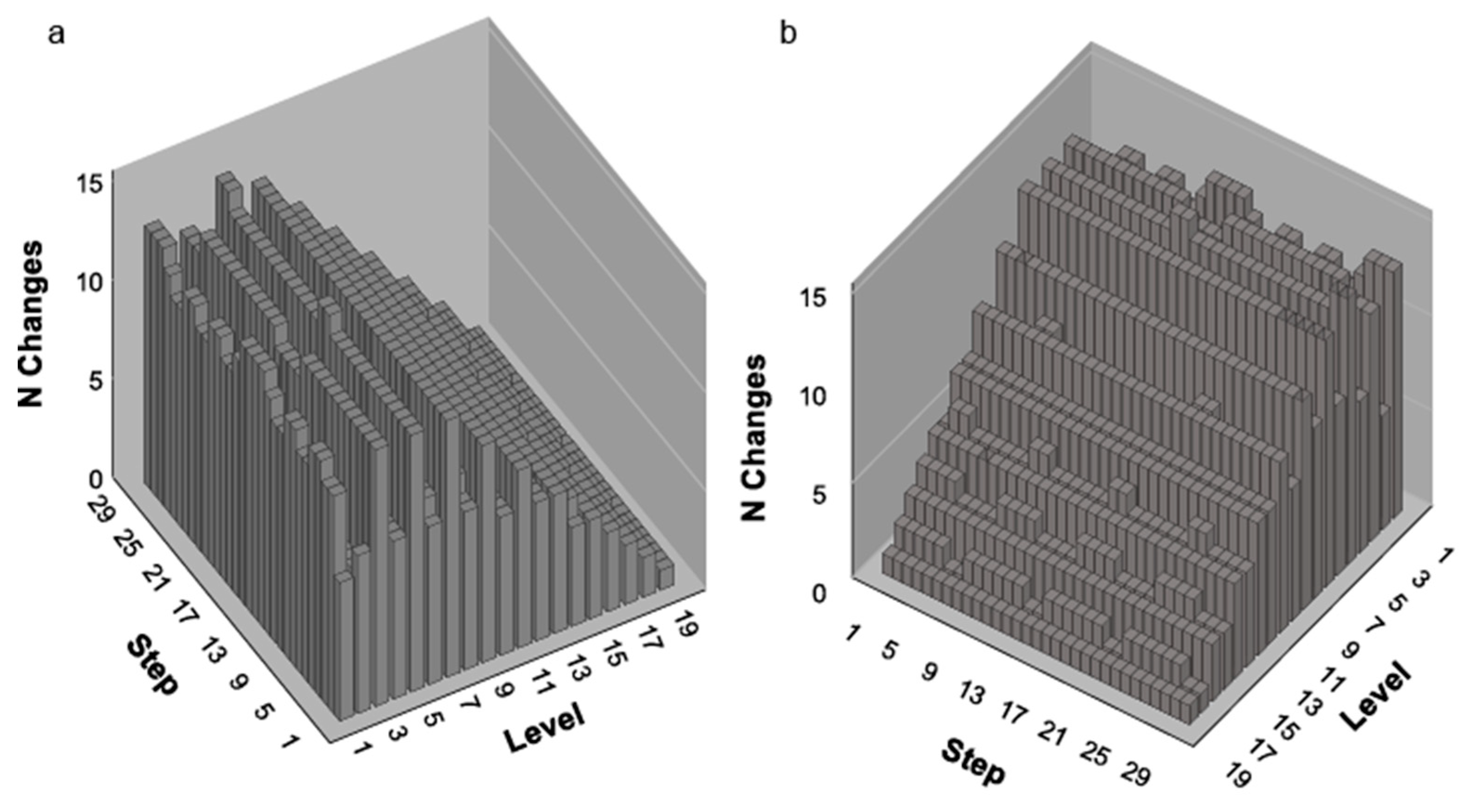
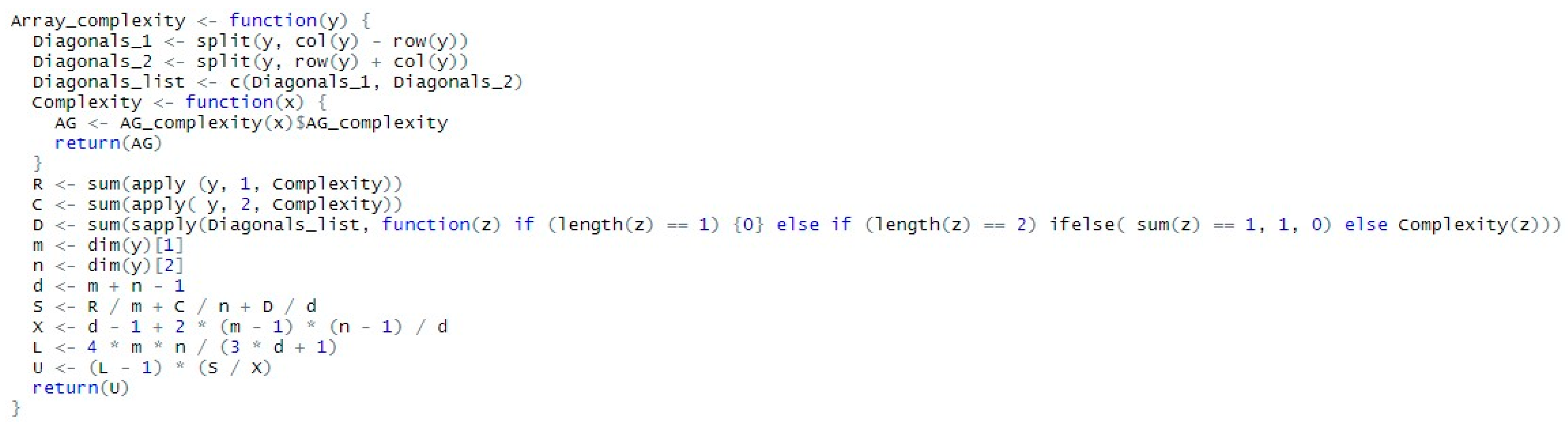
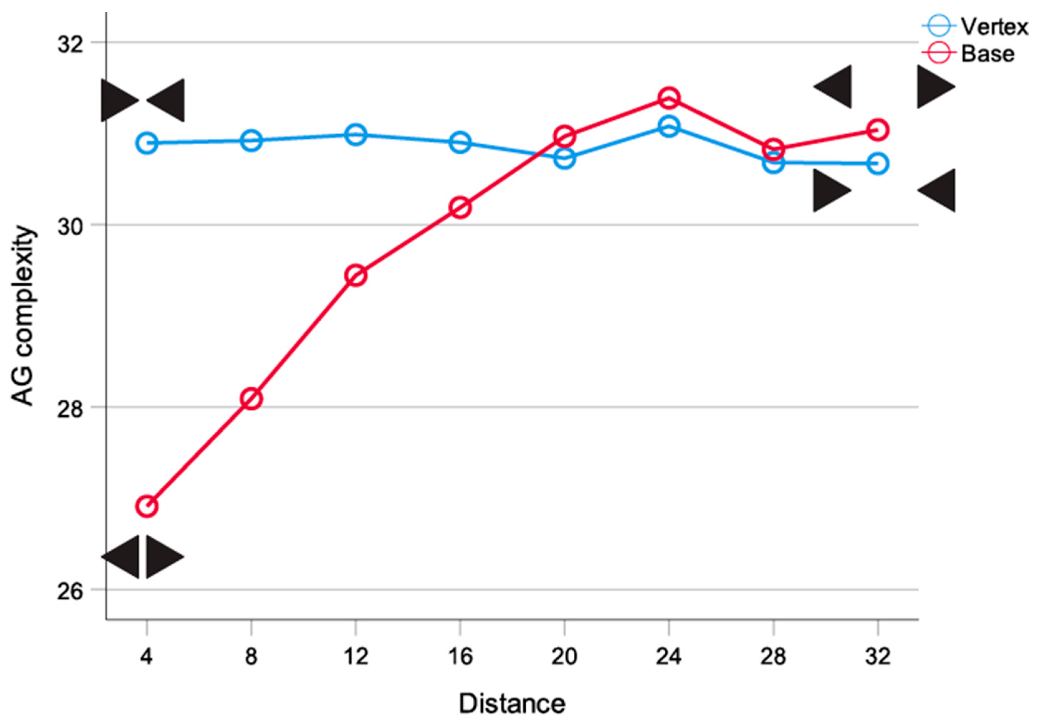
Table 1.
Correlations of AG and KC with subjective performance.
| Study | N (Patterns) | Mode | Presentation | Length | Measure | Correlation with AG | Correlation with KC a |
|---|---|---|---|---|---|---|---|
| Galanter & Smith (1958) | 6 | S | Seq | 2–5 | Prediction accuracy | 0.94 ** | 0.77 |
| Glanzer & Clark (1962) | 256 | V | Sim | 8 | Reproduction accuracy | −0.39 *** (−0.71 ***) | −0.18 * |
| Alexander & Carey (1967) | 35 | V | Sim | 7 | Overall goodness | −0.73 *** | 0.05 |
| Exp. 1 Search | −0.41 * | −0.15 | |||||
| Exp. 2 Sorting | −0.61 *** | 0.01 | |||||
| Exp. 3a Time | −0.58 *** | 0.19 | |||||
| Exp. 3b Confusion | −0.68 *** | −0.06 | |||||
| Exp. 4 Description | −0.68 *** | −0.06 | |||||
| Griffiths & Tenenbaum (2003) | 127 | V | Seq | 8 | Perceived randomness | 0.66 *** | 0.31 *** |
| Vitz (1968) | 26 | V | Seq | 1–8 | Judged complexity | 0.87 *** | 0.77 *** |
| Psotka (1975) | 35 | V | Seq | 8 | Judged complexity | 0.68 *** | −0.02 |
| Judged symmetry | −0.80 *** | −0.30 | |||||
| Judged syntely | −0.26 | 0.06 | |||||
| Garner & Gottwald (1967) | 10 | V | Seq | 5 | Trials to criterion | 0.75 * | −0.58 |
| Number of errors | 063† | −0.69 * | |||||
| Royer & Garner (1966) | 19 | A | Seq | 8 | Response uncertainty | 0.71 ** | 0.36 |
| Response delay | 0.69 ** | 0.40 † | |||||
| Error rate | 0.65 ** | 0.44 † | |||||
| 138 | Freq. SP | 0.09 | 0.02 | ||||
| Response delay | 0.49 *** | 0.20 * | |||||
| Error rate | 0.52 *** | 0.26 ** | |||||
| Falk & Kondold (1997) | 40 | V | Sim | 21 | Apparent randomness | 0.72 *** | 0.77 |
| Memorization difficulty | 0.79 *** | −0.18 * | |||||
| Copying difficulty | 0.80 *** | 0.05 | |||||
| Memorization time | 0.86 *** | −0.15 | |||||
| De Fleurian et al. (2016) | 48 | A | Seq | 49 | Correct ending | −0.32 * | 0.01 |
| Ease | −0.75 *** | 0.19 |
*** p < 0.001, ** p < 0.01, * p < 0.05, † p < 0.1A = Auditory, V = visual, S = speech; SP = starting pointa KC = CTM for strings under 13 bits; BDM for strings over 13 bits.
Table 2.
Strings selected from De Fleurian et al. 2016.
| String | Algorithm | KC |
|---|---|---|
| 10111011101110101011101110111010101110111011101010 | P16 | 0.00178 |
| 10110110101101010101101101010101101111010110101111 | GM | 0.0415 |
| 01010110100111011011111010110100101101111001100110 | B-0.5 | 0.0574 |
Note: KC = Kolmogorov complexity.
Table 3.
Correlations of 2D AG with complexity judgments.
| Study | N (Patterns) | Dimensions | Measure | Correlation with 2D AG |
|---|---|---|---|---|
| Chipman (1977) | 45 | 6 × 6 | Subjective complexity | 0.74 *** |
| Howe (1980) | 60 | 5 × 5 | Subjective goodness | 0.72 *** |
*** p < 0.001.
© 2020 by the authors. Licensee MDPI, Basel, Switzerland. This article is an open access article distributed under the terms and conditions of the Creative Commons Attribution (CC BY) license (http://creativecommons.org/licenses/by/4.0/).
Share and Cite
MDPI and ACS Style
Aksentijevic, A.; Mihailovic, A.; T. Mihailovic, D. Time for Change: Implementation of Aksentijevic-Gibson Complexity in Psychology. Symmetry 2020, 12, 948. https://doi.org/10.3390/sym12060948
AMA Style
Aksentijevic A, Mihailovic A, T. Mihailovic D. Time for Change: Implementation of Aksentijevic-Gibson Complexity in Psychology. Symmetry. 2020; 12(6):948. https://doi.org/10.3390/sym12060948
Chicago/Turabian StyleAksentijevic, Aleksandar, Anja Mihailovic, and Dragutin T. Mihailovic. 2020. "Time for Change: Implementation of Aksentijevic-Gibson Complexity in Psychology" Symmetry 12, no. 6: 948. https://doi.org/10.3390/sym12060948
Note that from the first issue of 2016, this journal uses article numbers instead of page numbers. See further details here.