1. Introduction
The bi-factor method of exploratory factor analysis (EFA) that was introduced by Holzinger and Swineford [
1] allows for identification of a general factor through all measured variables and several orthogonal group factors through sets of two or more measured variables. As explained by Holzinger and Swineford [
1] (p. 42), the general and group factors are uncorrelated “for economical measurement, simplicity, and parsimony”. Although offering interpretable solutions, bi-factor methods received less attention than multiple factor and higher-order factor models over the subsequent decades [
2,
3,
4,
5] and were not broadly applied in influential investigations of individual differences [
6,
7,
8,
9,
10,
11,
12].
Limitations of EFA methods and advances in theory and computer technology led to the ascendency of confirmatory factor analytic (CFA) methods that allow for testing hypotheses about the number of factors and the pattern of loadings [
13,
14]. Many CFA analyses have specified multiple correlated factors or higher-order models [
15,
16,
17,
18,
19,
20,
21,
22,
23]. Uniquely, Gustafsson and Balke [
24] applied what they termed a nested factor model, which was identical to the bi-factor model of Holzinger and Swineford [
1]. Subsequently, the bi-factor model has been recommended by Reise [
25] for CFA and successfully employed in the measurement of a variety of constructs, such as cognitive ability [
22], health outcomes [
26], quality of life [
27], psychiatric distress [
28], early academic skills [
29], personality [
30], psychopathology [
31], and emotional risk [
32].
Bi-factor models have been especially influential in research on human cognitive abilities because they frequently better fit the data than other models [
22] and because they instantiate a perspective that differs from that offered by other models [
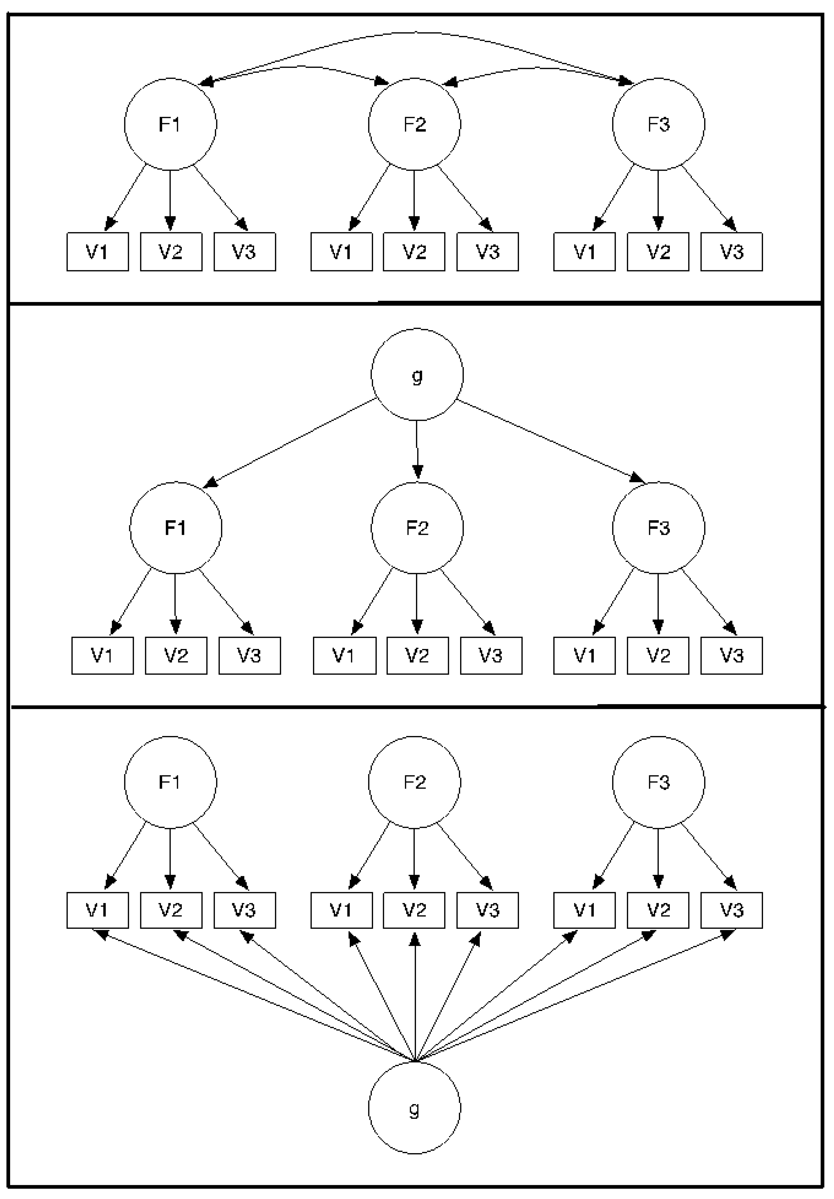
33]. As illustrated in the top panel of
Figure 1, a multiple correlated factors model does not include a general factor whereas both higher-order and bi-factor models include a general factor. As portrayed in the middle panel of
Figure 1, the general factor in a higher-order model is fully mediated by the lower-order factors. Thus, the general factor operates through the lower-order factors and only indirectly influences the measured variables. In contrast, the general factor in the bi-factor model (bottom panel) directly influences each measured variable independent of the influence exerted by the lower-order factors. The higher-order model is more constrained than the bi-factor model and is, therefore, mathematically nested within the bi-factor model [
34]. As nested models, fit comparisons via
difference tests are possible. Other fit indices, such as Akaike information criterion (AIC) and Bayesian information criterion (BIC) can also be used to compare the relative fit of the models, regardless of whether the models are nested or not.
An additional discussion of the relationship between these models is warranted. As stated previously, the bi-factor model and the second-order model are mathematically related. When proportionality constraints are imposed on the higher-order structure using the Schid-Leiman transformation, the bi-factor and higher-order structures are mathematically nested [
27]. Yung
et al. [
34] demonstrated using a generalized Schmid-Leiman transformation that the unrestricted higher-order (
i.e., items load directly onto first- and second-order factors) and bi-factor models are mathematically equivalent. The correlated factors model does not impose a measurement model on the first-order factors [
25] in that it does not specify a higher-order structure that explains the relationships between the first-order factors. Thus, the correlated factors model can be derived from a bi-factor model by constraining the general factor loadings to zero and relaxing the orthogonality constraint on the first-order factors [
25].
Figure 1.
Multiple correlated factor (top panel), higher-order (middle panel), and bi-factor (bottom panel) models.
Figure 1.
Multiple correlated factor (top panel), higher-order (middle panel), and bi-factor (bottom panel) models.
The bi-factor model has shown superior fit to models with first-order factors only [
35]; however, this was shown using item-level data rather than subscale-level data, which may be more relevant for intelligence test scores. Furthermore, the bi-factor model may be preferred when researchers hypothesize that specific factors account for unique influence of the specific domains over and above the general factor [
27].
Murray and Johnson [
36] recently questioned the propriety of statistical comparisons between bi-factor and higher-order models, suggesting that correlated residuals and cross-loadings (
i.e., misspecifications) may inherently bias such comparisons of fit indices in favor of the bi-factor model. They hypothesized that the bi-factor model parameters better absorb misspecification than higher-order parameters. To test their hypothesis, Murray and Johnson [
36] simulated three data sets of 500 subjects each with an underlying three-factor first-order structure based on parameters similar to those from a set of 21 cognitive tests. The first data set was without misspecification, the second included 6 correlated residuals at 0.1 and 3 cross-loadings at 0.2, and the third included 4 correlated residuals at 0.2, 6 correlated residuals at 0.1, and 6 cross-loadings at 0.2. Results showed that the bi-factor model exhibited superior fit to the data of the two simulation samples that contained misspecifications even though the true underlying structure was higher-order. In contrast, the comparative fit index (CFI), root mean square error of approximation (RMSEA), and standardized root mean square residual (SRMS) indices for bi-factor and higher-order models were identical for the sample without misspecifications. From these results, (Murray and Johnson [
36] p. 420) concluded that “the bi-factor model fits better, but not necessarily because it is a better description of ability structure”.
However, Murray and Johnson [
36] included a small number of parameters in their simulations and they did not generate “true” bi-factor or multiple correlated factors structure. Additionally, they only generated one data set for each set of parameters. As a consequence, there is no way to evaluate the influence of sampling error on their results. When using Monte Carlo methods, multiple iterations allow researchers to generate an empirical sampling distribution, which allows them to assess the average of random fluctuation (
i.e., error). Motivated by the Murray and Johnson [
36] study, we compared various fit indices for the bi-factor, higher-order, and correlated factors models when the underlying “true” structure was known to be one of the three models. Unlike Murray and Johnson [
36], misspecification (
i.e., correlated residuals and cross-loadings) beyond what the factor structure was able to account for was not included in our study because the additional model complexity would detract from our focus on fit index comparisons for true bi-factor, correlated factor, and higher-order factor models. Multiple correlated residuals and cross-loadings would indicate that the tested structure was insufficient for reproducing the observed covariance matrix. In that situation it would be reasonable to expect that a more general model would produce better statistical fit because the original model was already questionable [
37]. We varied parameters for each factor structure using subscale scores, and we generated 1000 replications of each set of parameters in a comparison of multiple correlated factors, higher-order, and bi-factor models.
3. Results
3.1. Convergence
Across all cells of the design, convergence was not problematic in that 98.9% of the solutions converged; however, all solutions that failed to converge were bi-factor solutions. Of the 405 solutions that did not converge, 374 were from data sets with 200 cases, and 31 were from data sets with 800 cases. Thus, sample size might be related to non-convergence of bi-factor models.
3.2. Models with Two Locally Just- and Two Locally Under-Identified Factors
We first compared the fit of competing models when two of the four factors each had only two indicators and the other two factors each had three indicators. The mean value of each approximate fit index across all conditions is presented in
Table 1. When the true underlying model was a bi-factor model, these indices tended to show that the bi-factor model fit better than the higher-order or correlated factors models. The percentage of solutions selected by each index for each cell of the study design is presented in
Table 2. Each index identified the bi-factor among the best fitting models more than 89% of the time with sample sizes of 200 and 100% of the time with sample sizes of 800. When only one of the three solutions was identified as the best fitting, each index tended to select the bi-factor solution over the higher-order or correlated factors models in at least 85% of the 200-case samples and 100% of the 800-case samples. The percentage of solutions selected by each index when only one model fit best for each cell of the study design is presented in
Table 3.
Table 4 shows the percentage of solutions identified by each of the information criteria. In samples of 200, both AIC and aBIC identified the bi-factor model as best fitting slightly more than half the time, and in samples of 800, AIC and aBIC identified the bi-factor model as best fitting in 90% of the samples or higher. BIC imposes a harsher penalty for model complexity than AIC or aBIC so it identified the higher-order solution as best fitting more frequently than the true bi-factor although to a lesser extent with sample of 800 than 200.
When the true underlying model was the multiple correlated factors model, the fit indices tended to show that the correlated factors model fit better than the higher-order or bi-factor models. The CFI, TLI, and RMSEA identified the correlated factors model among the best fitting at least 86% of the time with sample sizes of 200 and 99% of the time with sample sizes of 800. Overall, the SRMR identified the correlated factors model among the best fitting 73% of the time, but it was impacted by sample size. In sample sizes of 200, SRMR identified the bi-factor and/or correlated factors solutions among the best fitting 56% and 51% of the time, respectively. However, in sample sizes of 800, SRMR identified the bi-factor and/or correlated factors solutions among the best fitting 12% and 92% of the time, respectively. When only one of the three solutions was identified as the best fitting, CFI, TLI, and RMSEA tended to select the correlated factors solution at least 92% of the time over the higher-order or bi-factor models. Among the information criteria, all three identified the correlated factor model as best fitting in at least 81% of the samples of size 200 and 99% of the samples of size 800.
Table 1.
Mean values for each approximate fit index for each cell of the study design.
Table 1.
Mean values for each approximate fit index for each cell of the study design.
Indicators
Per
Factor | Sample
Size | True
Model | Fitted Model |
|---|
| Bi-Factor | | Correlated Factors | | Higher-Order |
|---|
| CFI | TLI | RMSEA | SRMR | | CFI | TLI | RMSEA | SRMR | | CFI | TLI | RMSEA | SRMR |
|---|
3:1;
2:1 | 200 | Bi | 0.997 | 1.000 | 0.015 | 0.021 | | 0.990 | 0.986 | 0.040 | 0.038 | | 0.982 | 0.975 | 0.055 | 0.127 |
| CF | 0.991 | 0.988 | 0.027 | 0.033 | | 0.995 | 0.999 | 0.016 | 0.016 | | 0.974 | 0.964 | 0.049 | 0.089 |
| H-O | 0.997 | 0.991 | 0.016 | 0.029 | | 0.994 | 0.994 | 0.023 | 0.035 | | 0.991 | 0.988 | 0.031 | 0.063 |
| 800 | Bi | 0.999 | 1.000 | 0.008 | 0.010 | | 0.991 | 0.986 | 0.042 | 0.031 | | 0.983 | 0.976 | 0.057 | 0.123 |
| CF | 0.994 | 0.990 | 0.026 | 0.021 | | 0.999 | 1.000 | 0.007 | 0.016 | | 0.975 | 0.965 | 0.052 | 0.064 |
| H-O | 0.999 | 1.000 | 0.007 | 0.014 | | 0.997 | 0.996 | 0.018 | 0.022 | | 0.993 | 0.990 | 0.032 | 0.055 |
| 3:1 | 200 | Bi | 0.997 | 0.999 | 0.014 | 0.022 | | 0.994 | 0.993 | 0.025 | 0.028 | | 0.985 | 0.980 | 0.045 | 0.011 |
| CF | 0.990 | 0.988 | 0.025 | 0.036 | | 0.995 | 0.999 | 0.014 | 0.034 | | 0.975 | 0.968 | 0.042 | 0.090 |
| H-O | 0.997 | 0.999 | 0.014 | 0.031 | | 0.996 | 0.999 | 0.014 | 0.033 | | 0.992 | 0.991 | 0.024 | 0.063 |
| 800 | Bi | 0.999 | 1.000 | 0.007 | 0.011 | | 0.996 | 0.994 | 0.026 | 0.018 | | 0.986 | 0.981 | 0.047 | 0.108 |
| CF | 0.993 | 0.989 | 0.025 | 0.024 | | 0.999 | 1.000 | 0.007 | 0.017 | | 0.976 | 0.970 | 0.047 | 0.083 |
| H-O | 0.999 | 1.000 | 0.007 | 0.015 | | 0.999 | 1.000 | 0.006 | 0.016 | | 0.994 | 0.992 | 0.026 | 0.052 |
Table 2.
Percentage of solutions selected by each approximate fit index for each cell of the study design (rounded to nearestwhole number).
Table 2.
Percentage of solutions selected by each approximate fit index for each cell of the study design (rounded to nearestwhole number).
Indicators
Per
Factor | Sample
Size | True
Model | Fitted Model |
|---|
| Bi-Factor | | Correlated Factors | | Higher-Order |
|---|
| CFI | TLI | RMSEA | SRMR | | CFI | TLI | RMSEA | SRMR | | CFI | TLI | RMSEA | SRMR |
|---|
3:1;
2:1 | 200 | Bi | 94 | 91 | 89 | 99 | | 14 | 14 | 13 | 1 | | 36 | 37 | 35 | 2 |
| CF | 42 | 38 | 37 | 56 | | 86 | 87 | 86 | 51 | | 43 | 42 | 41 | 7 |
| H-O | 72 | 67 | 67 | 70 | | 70 | 71 | 79 | 37 | | 65 | 66 | 65 | 6 |
| 800 | Bi | 100 | 100 | 100 | 100 | | 0 | 0 | 0 | 0 | | 4 | 4 | 2 | 0 |
| CF | 9 | 7 | 6 | 12 | | 99 | 99 | 99 | 92 | | 8 | 8 | 7 | 3 |
| H-O | 80 | 71 | 65 | 76 | | 79 | 79 | 71 | 36 | | 79 | 77 | 67 | 9 |
| 3:1 | 200 | Bi | 91 | 86 | 85 | 97 | | 33 | 33 | 30 | 6 | | 30 | 33 | 31 | 0 |
| CF | 38 | 35 | 34 | 38 | | 89 | 90 | 90 | 71 | | 33 | 35 | 33 | 0 |
| H-O | 72 | 66 | 64 | 71 | | 66 | 65 | 62 | 36 | | 68 | 71 | 68 | 0 |
| 800 | Bi | 100 | 100 | 100 | 100 | | 3 | 2 | 1 | 0 | | 3 | 2 | 1 | 0 |
| CF | 4 | 4 | 3 | 2 | | 99 | 100 | 99 | 99 | | 5 | 4 | 3 | 0 |
| H-O | 83 | 73 | 66 | 77 | | 83 | 79 | 66 | 36 | | 80 | 82 | 72 | 0 |
Table 3.
Percentage of solutions selected by each approximate fit index when only one model fit best for each cell of the study design (rounded to nearest whole number).
Table 3.
Percentage of solutions selected by each approximate fit index when only one model fit best for each cell of the study design (rounded to nearest whole number).
Indicators
Per
Factor | Sample
Size | True
Modle | Fitted Model |
|---|
| Bi-Factor | | Correlated Factors | | Higher-Order |
|---|
| CFI | TLI | RMSEA | SRMR | | CFI | TLI | RMSEA | SRMR | | CFI | TLI | RMSEA | SRMR |
|---|
3:1;
2:1 | 200 | Bi | 91 | 87 | 85 | 99 | | 2 | 3 | 4 | 1 | | 6 | 10 | 11 | 0 |
| | (654) | (665) | (702) | (947) | | | | | | | | | | |
| CF | 13 | 11 | 11 | 50 | | 79 | 80 | 79 | 50 | | 8 | 9 | 9 | 0 |
| | | | | | | (501) | (512) | (533) | (737) | | | | | |
| H-O | 46 | 37 | 37 | 67 | | 37 | 40 | 39 | 32 | | 18 | 23 | 24 | 1 |
| | | | | | | | | | | | (401) | (415) | (443) | (885) |
| 800 | Bi | 100 | 100 | 100 | 100 | | 0 | 0 | 0 | 0 | | 0 | 0 | 0 | 0 |
| | (958) | (964) | (981) | (1000) | | | | | | | | | | |
| CF | 1 | 1 | 1 | 7 | | 99 | 99 | 99 | 94 | | 0 | 0 | 0 | 0 |
| | | | | | | (895) | (907) | (920) | (925) | | | | | |
| H-O | 45 | 35 | 34 | 70 | | 36 | 42 | 39 | 30 | | 19 | 23 | 27 | 0 |
| | | | | | | | | | | | (229) | (273) | (429) | (814) |
| 3:1 | 200 | Bi | 90 | 85 | 83 | 97 | | 7 | 8 | 9 | 3 | | 3 | 7 | 8 | 0 |
| | (678) | (686) | (717) | (957) | | | | | | | | | | |
| CF | 14 | 10 | 11 | 32 | | 84 | 85 | 85 | 68 | | 2 | 4 | 4 | 0 |
| | | | | | | (531) | (538) | (552) | (751) | | | | | |
| H-O | 54 | 43 | 40 | 69 | | 24 | 24 | 25 | 31 | | 22 | 32 | 35 | 0 |
| | | | | | | | | | | | (389) | (412) | (475) | (930) |
| 800 | Bi | 100) | 100 | 100 | 100 | | 0 | 0 | 0 | 0 | | 0 | 0 | 0 | 0 |
| | (968) | (973) | (988) | (1000) | | | | | | | | | | |
| CF | 1 | 0 | 1 | 1 | | 99 | 100 | 99 | 99 | | 0 | 0 | 0 | 0 |
| | | | | | | (928) | (931) | (942) | (976) | | | | | |
| H-O | 62 | 48 | 40 | 73 | | 26 | 26 | 25 | 27 | | 12 | 26 | 34 | 0 |
| | | | | | | | | | | | (195) | (227) | (409) | (874) |
Table 4.
Percentage of solutions selected by each information criterion (rounded to nearest whole number).
Table 4.
Percentage of solutions selected by each information criterion (rounded to nearest whole number).
Indicators
Per
Factor | Sample
Size | True
Model | Fitted Model |
|---|
| Bi-Factor | | Correlated Factors | | Higher-Order |
|---|
| AIC | BIC | aBIC | | AIC | BIC | aBIC | | AIC | BIC | aBIC |
|---|
3:1;
2:1 | 200 | Bi | 55 | 4 | 51 | | 7 | 12 | 7 | | 38 | 84 | 41 |
| CF | 2 | 0 | 2 | | 81 | 83 | 81 | | 16 | 17 | 16 |
| H-O | 9 | 0 | 8 | | 48 | 50 | 48 | | 43 | 50 | 44 |
| 800 | Bi | 99 | 45 | 90 | | 0 | 0 | 0 | | 1 | 55 | 10 |
| CF | 0 | 0 | 0 | | 99 | 99 | 99 | | 1 | 1 | 1 |
| H-O | 7 | 0 | 1 | | 50 | 52 | 52 | | 44 | 48 | 48 |
| 3:1 | 200 | Bi | 39 | 0 | 34 | | 9 | 1 | 8 | | 51 | 99 | 58 |
| CF | 1 | 0 | 1 | | 74 | 24 | 72 | | 25 | 76 | 27 |
| H-O | 5 | 0 | 4 | | 14 | 0 | 12 | | 81 | 100 | 84 |
| 800 | Bi | 98 | 9 | 77 | | 1 | 0 | 1 | | 1 | 91 | 22 |
| CF | 0 | 0 | 0 | | 100 | 90 | 99 | | 0 | 10 | 1 |
| H-O | 4 | 0 | 0 | | 14 | 0 | 4 | | 82 | 100 | 97 |
When the true underlying model was the higher-order model, the fit indices did not show the same tendencies of preferring the true underlying model. The CFI identified the bi-factor solution most often (76%), TLI identified the correlated factors solution most often (75%), RMSEA identified the higher-order solution most often (66%), and SRMR identified the bi-factor solution most often (73%) among the best fitting models. The performance of the fit indices is more easily interpreted when considering the datasets for which only one solution was identified as best because the percentages must sum to 100% within rounding error (see
Table 3). Across all cells of the design with two under-/two just-identified factors, CFI identified the bi-factor solution most frequently (45%) followed by the correlated factors solution (37%) and higher-order solution (18%). For TLI, the correlated factors solution was identified most frequently (41%) followed by the bi-factor solution (36%) and higher-order solution (23%). For RMSEA, the correlated factors solution was identified most frequently (39%) followed by the bi-factor solution (35%) and higher-order solution (25%). For SRMR, the bi-factor solution was identified most frequently (68%) followed by the correlated factors solution (31%) and higher-order solution (0%). The fit index performance under the true higher-order conditions were not as heavily impacted by sample size as for the other true models. The identification of best fitting models by the information criteria was fairly evenly split between the higher-order and correlated factor models (see
Table 4).
3.3. Models with Four Locally Just-Identified Factors
Next, we compared the fit of competing models when all four factors were measured by three indicators each. The mean value of each fit index across all conditions is presented in
Table 1. When the true underlying model was a bi-factor model, the fit indices tended to favor the bi-factor solution over the higher-order or correlated factors solutions. The percentage of solutions selected by each index for each cell of the study design is presented in
Table 2. Each index identified the bi-factor among the best fitting models more than 85% of the time with sample sizes of 200 and 100% of the time with sample sizes of 800. When only one of the three solutions was identified as the best fitting, each index tended to select the bi-factor solution over the higher-order or correlated factors models in at least 83% of the 200-case samples and 100% of the 800-case samples. The percentage of solutions selected by each index when only one model fit best for each cell of the study design is presented in
Table 3. Of the information criteria, BIC almost exclusively identified the higher-order model as the best fitting model across sample sizes. AIC and aBIC identified the higher-order model as the best fitting in just over half of the true bi-factor samples of size 200 and in over 80% of the samples of size 800.
When the true underlying model was a multiple correlated factors model, the approximate fit indices tended to favor the bi-factor solution. Each index identified the bi-factor among the best fitting models more than 70% of the time with sample sizes of 200 and 99% of the time with sample sizes of 800. When only one of the three solutions was identified as the best fitting, each index tended to select the bi-factor solution over the higher-order or correlated factors models in at least 68% of the 200-case samples and 99% of the 800-case samples. Among the information criteria, AIC and aBIC identified the correlated factors model as the best fitting in about 75% of the cases and for nearly all of the samples of size 200 and 800, respectively. In the larger sample size condition, BIC identified the correlated factors model as the best fitting in 90% of the samples but in only 24% of the samples of size 200. Instead, BIC tended to identify the higher-order as the best fitting model in about 75% of the samples.
When the true underlying model was a higher-order model, the approximate fit indices were mixed when considering all of the conditions together. In about half of the datasets, CFI, TLI, and RMSEA showed that all three solutions fit the data equally well. This finding was expected given that the higher-order model is a constrained version of the correlated factors and bi-factor models. Based on SRMR, the higher-order solution did not fit as well or better than the bi-factor or correlated factors solutions in any of these datasets. In cases where one solution fit better than the other two, all four fit indices tended to prefer the bi-factor solution but to different degrees. For CFI, the bi-factor solution was identified most frequently (57%) followed by the correlated factors solution (25%) and higher-order solution (18%). For TLI, the bi-factor solution was identified most frequently (45%) followed by the higher-order solution (30%) and correlated factors solution (25%). For RMSEA, the bi-factor solution was identified most frequently (40%) followed by the higher-order solution (35%) and correlated factors solution (25%). For SRMR, the bi-factor solution was identified most frequently (61%) followed by the correlated factors solution (29%). The fit index performance under the true higher-order conditions were not as heavily impacted by sample size as for the other true models. In contrast, the information criteria tended to identify the higher-order model in at least 81% of the samples and BIC identified the higher-order model in all of the samples generated in this study.
3.4. Summary
These findings suggest that when data were sampled from a population with a true bi-factor structure, each of the approximate fit indices examined here was more likely than not to identify the bi-factor solution as the best fitting out of the three competing solutions. However, only AIC and aBIC tended to identify the bi-factor solution when sample sizes were larger. BIC tended to identify the higher-order solution regardless of sample size. When samples were selected from a population with a true multiple correlated factors structure, CFI, TLI, and RMSEA were more likely to identify the correlated factors solution as the best fitting out of the three competing solutions. With a large enough sample size, SRMR was also likely to identify the correlated factors model. AIC and aBIC tended to identify the correlated factors solution regardless of sample size, and BIC only performed well in larger sample sizes. When samples were generated from a population with a true higher-order structure, each of the fit indices tended to identify the bi-factor solution as best fitting instead of the true higher-order model. The SRMR had the strongest tendency to prefer the bi-factor model, which was expected because less parsimonious models allow more parameters to be freely estimated, which typically produce better statistical fit than more parsimonious models. Unlike the CFI, TLI, and RMSEA, the SRMR does not penalize the bi-factor model for being less parsimonious than the higher-order model. Each of the information criteria tended to correctly identify the higher-order model when there were at least three indicators per factor. This again should be expected because the differences in parsimony between these models increases as more indicators are added. In summary, our study shows that approximate fit indices and information criteria should be very cautiously considered when used to aid in model selection. Substantive and conceptual grounds should be more heavily weighted in the model selection decision.
4. Discussion
Previous research has suggested that the fit indices may statistically favor the bi-factor model [
36] as compared with the higher-order model in CFA studies of cognitive abilities when model violations (e.g., correlated residuals, cross-loadings) are present. In the current study, the bi-factor model did not generally produce a better fit when the true underlying structure was not a bi-factor one. However, there was considerable overlap of fit values across the models. For example, with a sample size of 200 and under-identified factors the average CFI values of bi-factor and higher-order models were 0.997 and 0.991, respectively, when the true structure was higher-order. In that same condition, the average RMSEA values of bi-factor and higher-order models were 0.016 and 0.031, respectively. There was almost total overlap of fit with a sample size of 800 and a factor to variable ratio of 1:3: the average CFI value of a true higher-order structure was 0.999 for a bi-factor model, 0.999 for a correlated factors model, and 0.994 for a higher-order model. In contrast, the RMSEA values for these three models were 0.007, 0.006, and 0.026, respectively.
Given previous research on the relationships between these models [
25,
34], the bi-factor model would be expected to result in the best fit because it is the most general (
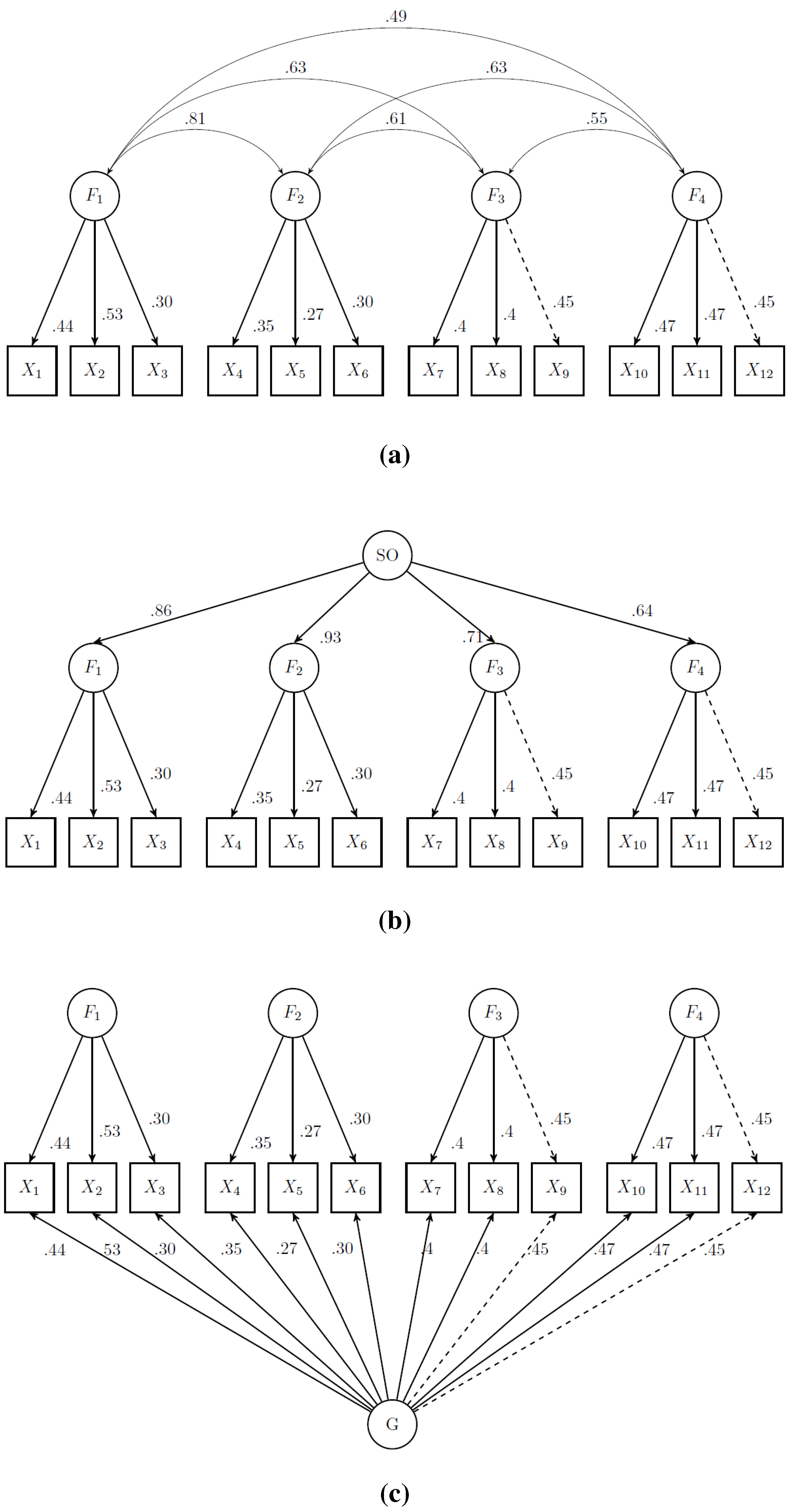
i.e., least restrictive) model examined. The present study demonstrated that CFA fit indices are sensitive to differences in the true underlying models at least under the conditions that were simulated. That is, the fit indices tended to identify the multiple correlated factors model in most of the datasets that were selected from populations in which the correlated factors structure was true. As shown in
Figure 2, the correlations specified between the factors in correlated factors models were somewhat discrepant. In other words, all factors were not correlated equally strongly with each other pairwise. Under the bi-factor model, a general factor accounted for whatever correlations were observed between factors. When the factor correlations were not equal, then the general factor was not able to equally account for the correlation between the specific factors. In such a case, the general factor was not really functioning as a general factor; rather, it was functioning as a general factor for a subset of specific factors. Interested readers should see Carroll [
48] for a more detailed discussion of correlated factors and the discovery of general factors. Unlike the bi-factor model, the correlated factors model was readily able to allow the strength of correlations between factors to vary. As a result, the bi-factor model was unlikely to fit best when the factor correlations were unequal. Given that the population parameters used in this study were taken from applied studies of cognitive abilities, equal factor correlations may be unrealistic in applied research settings.
Model selection using the fit indices was strongly related to differences in the number of estimated parameters (
i.e., model complexity) between the models. Generally speaking, more complex models tend to fit data better than less complex models, but the improvement in fit must be substantial enough to justify the estimation of more parameters. In the samples with 10 indicators, the bifactor model had 38 estimated parameter compared with 34 for the correlated factors and higher-order models. CFI, TLI, and the information criteria incorporate and adjust for model complexity. For the true bi-factor samples with 10 indicators, the improvement in fit of the bi-factor model was generally enough to justify estimating only four more parameters. For the true correlated factors samples with 10 indicators, the improvement in fit of the bi-factor model was generally not enough to justify estimating four more parameters. Yet, the correlated factors model and higher-order model required the same number of parameters to be estimated so one might reasonably expect the it would not be identified as the best fitting as frequently because it is more restrictive than the correlated factors or bi-factor model. A numerical example may help illustrate the relationship between model complexity and fit. Consider the equation for CFI in Equation (
1).
where
is the
value for the tested model,
is the degrees of freedom of the tested model,
is the
value for the null model (
i.e., no covariances are specified), and
is the degrees of freedom for the null model. For a randomly selected replication from the true higher-order model, the values needed for computing CFI are:
,
,
, and
. The estimated CFI is 0.997. Suppose the bi-factor model was also estimated, and it fit equally well in absolute terms (
i.e.,
). The null model remains the same (
i.e.,
,
) for the bi-factor model, but the degrees of freedom are different for the bi-factor model (
) because it requires more parameters to be estimated over the higher-order model. Using these values, the estimated CFI for the bi-factor model is 0.995. Even though the models fit exactly the same in absolute terms, CFI penalizes the bi-factor model more heavily because it is less parsimonious. In this case, the additional parameter estimates are not worth the added model complexity because the fit did not improve enough to result in better model-data fit. This trade-off between parsimony and model fit becomes more and more apparent in the models with more indicators. In the numerical example above, 12 indicators were used, which resulted in a difference of eight estimated parameters (
). As more indicators are used, the difference in estimated parameters becomes more discrepant. For example, the numbers of parameters required for the models with, say, 20 indicators would be 80 for the bi-factor model, 64 for the correlated factors model, and 62 for the higher-order factor model.
Additional attention should also be given to another aspect of model complexity, which was central to the simulation design in Murray and Johnson [
36]. They added varying degrees of model complexity in the form of correlated residuals and cross-loading items to examine the sensitivity of the competing models to model misspecification. We elected not to build unmodeled complexity and/or misspecification into our study’s design because ours was an initial investigation into fit index comparisons under conditions found in the extant literature. Of course, cross-loadings and residual covariances may be encountered in applied settings, but they were not reported in the studies we reviewed. Furthermore, small and/or nonsubstantive model complexity may occasionally occur due to random sampling error, but this is quite different from generating data on the basis of correlated errors and cross-loadings. For example, in a randomly selected replication from one of our true higher-order model conditions, we observed residuals between various indicators that were correlated at around 0.1 and cross-loadings at around 0.15, which is consistent with Murray and Johnson’s [
36] discussion. Again, we should note that the mechanism responsible for the small model complexities in this study and [
36] are different. Because we replicated each condition many times, we were able to rule out the effect that such residual correlations and cross-loadings had on fit index performance in the long run because there was no unmodeled complexity, on average, across thousands of replications. Finally, the conditions generated by Murray and Johnson [
36] may also be representative of those conditions that applied researchers are likely to encounter. An extension of their work with an increased number of replications would be helpful for further examining the potential bias in fit and/or parameter estimates that favor the bi-factor model because it would help control for random sampling error.
However, simulations as scientific proof have limitations [
49] and the exclusive use of approximate fit statistics is perilous [
46]. As concluded by (McDonald [
50] p. 684), “if the analysis stops at the globally fitted model, with global approximation indices, it is incomplete and uninformative”. Each of the tested models offers a different perspective on the structure of cognitive abilities [
33,
51] that should guide the researcher. As noted by Murray and Johnson [
36], to avoid misinterpretation of resulting ability estimates, the purpose of the measurement model must be taken into account. For example, a correlated factors model does not contain a general factor and attributes all explanatory variance to first-order factors, a higher-order model posits that the general factor operates only through the first-order factors and thereby conflates the explanatory variance of general and first-order factors, and a bi-factor model disentangles the explanatory variance of general and first-order factors but does not allow the general factor to directly influence the first-order factors. Thus, approximate fit statistics are useful but not dispositive [
46].


