Learning of temporal motor patterns: an analysis of continuous versus reset timing
- 1 Department of Neurobiology, University of California, Los Angeles, CA, USA
- 2 Departamento de Ciencia y Tecnología, Universidad Nacional de Quilmes, Bernal, Argentina and CONICET, Argentina
- 3 Department of Psychology and Brain Research Institute, University of California, Los Angeles, CA, USA
Our ability to generate well-timed sequences of movements is critical to an array of behaviors, including the ability to play a musical instrument or a video game. Here we address two questions relating to timing with the goal of better understanding the neural mechanisms underlying temporal processing. First, how does accuracy and variance change over the course of learning of complex spatiotemporal patterns? Second, is the timing of sequential responses most consistent with starting and stopping an internal timer at each interval or with continuous timing? To address these questions we used a psychophysical task in which subjects learned to reproduce a sequence of finger taps in the correct order and at the correct times – much like playing a melody at the piano. This task allowed us to calculate the variance of the responses at different time points using data from the same trials. Our results show that while “standard” Weber’s law is clearly violated, variance does increase as a function of time squared, as expected according to the generalized form of Weber’s law – which separates the source of variance into time-dependent and time-independent components. Over the course of learning, both the time-independent variance and the coefficient of the time-dependent term decrease. Our analyses also suggest that timing of sequential events does not rely on the resetting of an internal timer at each event. We describe and interpret our results in the context of computer simulations that capture some of our psychophysical findings. Specifically, we show that continuous timing, as opposed to “reset” timing, is consistent with “population clock” models in which timing emerges from the internal dynamics of recurrent neural networks.
Introduction
The nervous system processes and tracks time over a range of at least 12 orders of magnitude: from our ability to discriminate whether sounds arrive at our left or right ear first (microseconds), to the governing of our circadian rhythms (hours and days). In between these extremes, on the order of milliseconds and seconds, lie what might be considered the most sophisticated forms of timing: those that are required for complex sensory and motor tasks, including speech, or music, perception, and production. It is clear that, unlike the clocks on our wrists or walls that can be used to track milliseconds or months, the brain uses fundamentally different mechanisms to time across different scales (Lewis et al., 2003; Mauk and Buonomano, 2004; Buhusi and Meck, 2005; Buonomano, 2007; Grondin, 2010). For example, the axonal delay lines that contribute to sound localization (Jeffress, 1948; Carr, 1993) have nothing to do with the transcription/translation feedback loops that govern circadian rhythms (King and Takahashi, 2000; Panda et al., 2002). Indeed, while significant progress has been made toward understanding the mechanisms underlying timing in the extremes of biological temporal processes, less progress has been made toward elucidating the mechanism, or more likely mechanisms, underlying timing the in range of hundreds of milliseconds to a few seconds. It is this range, with particular attention to the motor domain, which will be the focus of the current paper.
As in many other areas of sensory perception, Weber’s Law has maintained a dominant presence in the field of temporal processing. Specifically, that the SD of motor responses or the precision of sensory discrimination varies linearly with absolute interval. In other words, the coefficient of variation (CV, or Weber’s fraction), defined as the SD over mean time, should be constant. This linear relationship is often referred to as the scalar property (Gibbon, 1977).
There is excellent evidence that Weber’s law holds true over certain time scales in some paradigms (Gibbon, 1977; Meck and Church, 1987; Allan and Gibbon, 1991; Church et al., 1994; Hinton and Rao, 2004; Jazayeri and Shadlen, 2010). However it is also clear that, at least in its simplest form, Weber’s law does not universally hold true. For example, Lewis and Miall (2009) recently reported that in a time reproduction task over a range of 68 ms to 16 min there was a progressive decrease in the CV; they concluded “this finding joins other recent reports in demonstrating a systematic violation of the scalar property in timing data.” Indeed, many studies have stressed that even within narrow time ranges both sensory (Getty, 1975; Hinton and Rao, 2004) and motor (Ivry and Hazeltine, 1995; Bizo et al., 2006; Merchant et al., 2008) timing violates Weber’s law. However, these data seem to be well accounted for by a generalized form of Weber’s law (Getty, 1975; Ivry and Hazeltine, 1995; Bizo et al., 2006; Merchant et al., 2008), in which the variance increases as T2 plus a time-independent (residual or noise) variance component. The time-dependent component of the variance is often interpreted as reflecting the properties of some “internal clock,” while the independent term is often viewed as reflecting with motor variability. Few, if any, studies have explicitly quantified how these different components change with learning. Here we show that both components change during learning.
Interestingly the majority of studies that have explicitly quantified the relationship between variance and time have done so using independent intervals. That is, the variance of distinct intervals, such as the production of 0.5, 1, and 2 s intervals, is analyzed in separate trials. Here we use a spatiotemporal (or purely temporal) pattern reproduction task, in which the accuracy and precision to multiple consecutive responses within a pattern can be obtained within the same trial. We first confirm that even within a fairly narrow range of a few seconds, the standard version of Weber’s law (constant CV) is violated; however, the generalized version where variance increases in proportion to T2 captures the data well. Additionally, this task allowed us to address a specific question relating to the timing of consecutive intervals. Consider a temporal task such as pressing a sequence of keys on a piano at the appropriate times. Does this task rely on timing all consecutive events in relation to the sequence onset time (t = 0), or on resetting and restarting an internal timer at each event – and thus essentially consist of timing consecutive intervals in isolation? Based on expected differences in the variability signature of consecutive responses we conclude that the “internal timer” is not reset during each event.
Finally, based on a previously presented model, we demonstrate how recurrent neural networks that do not exhibit any periodic clock-like activity can generate complex spatiotemporal patterns. The model is consistent with non-resetting timing mechanisms; however, we also highlight the need for this and other models to quantitatively account for the experimentally observed variance characteristics.
Materials and Methods
Tasks
The basic task used in this work resembles playing a melody on a piano, by pressing the correct keys in the correct order and target times. Two versions of the task were used: a spatiotemporal pattern reproduction (STPR) task (Experiment 1), where the subjects used four fingers to press the corresponding keys on a computer keyboard; and a Temporal Pattern Reproduction (TPR) task (Experiment 2) where the subjects used only one finger and one key. In the STPR version, each of four rectangles on a computer screen is assigned a corresponding computer key and finger: keys F-D-S-A were assigned to fingers 2 (index) through 5 (pinky) of the left hand. Subjects learned a spatiotemporal pattern consisting of a sequence of key presses; the spatial component corresponds to the order in which each key must be pressed, and the temporal component to the time each key must be pressed in relation to t = 0. Each trial consisted of an exposure component followed by a training/testing component. The exposure component is similar to a “temporal” serial reaction time task (Nissen and Bullemer, 1987; Shin and Ivry, 2002): the subject is instructed to press the appropriate key in response to every flashed rectangle. Stimuli were presented in “open-loop” mode, i.e., the events continue independent of if and when the subject responds. After the exposure component, the training/testing component begins with an onset cue, and then the subject is required to reproduce the entire spatiotemporal pattern on their own as accurately as possible; in this phase the rectangles appear only if and when the subject presses one of the four keys. The beginning of the pattern (t = 0) was initiated by the subject by pressing the space bar with the thumb. The response time of each key press in relation to t = 0 is recorded to calculate the variance, root-mean-square error (RMSE), and mean of the response times for further analysis. Feedback on the training/testing component is provided at the end of each trial in the form of a performance index, and an image of a “raster” that illustrates the target and produced patterns. In the TPR version of the task only one key/finger was used to reproduce the entire pattern (i.e., a purely temporal pattern with no spatial component). In this task, in an attempt to minimize previous experience all subjects used their pinky finger (left hand).
General Procedure
During the test subjects sat in front of a computer monitor with a keyboard in a quiet room. Stimulus presentation and behavioral response collection were controlled by a personal computer using custom-written code in Matlab and PsychToolBox. As the overall performance measure to track learning we used the RMSE between the response times and the target times.
Weber’s Generalized Law
We fit the “Weber generalized law” (Eq. 1) to our data; and to provide a comparison we also performed fits using a related equation with the same number of degrees of freedom where variance was a linear function of T (Eq. 2; Ivry and Hazeltine, 1995). Specifically:
where σ2 represents the total variance,  the time-independent variance, and k (in Eq. 1) approximates the square root of the conventional Weber fraction at long intervals. Both equations predict a decreasing CV as a function of absolute time T, although to differing degrees.
Slope and Intercept of the Generalized Weber’s Law
For every day and every subject classified as a learner (see Experiment 1), we performed a linear regression between the variance of each response time and the mean absolute response times squared throughout the pattern. The fitted slope and intercept of the linear regression were the estimates for the parameters k and  in the equation for the generalized Weber’s law above (Eq. 1).
Reset versus Continuous Timing
To examine the Reset versus Continuous timing hypotheses we fit two different functions to the data. Consider the responses to a temporal pattern composed of six consecutive intervals t1…t6, so that the absolute timing of each response is T1…T6, with T1 = t1, T2 = t1 + t2,…,T6 = t1 + t2 + … + t6. The Reset Timing hypothesis assumes that the variance at each response along the pattern adds to the accumulated variance from previous responses, so that the variance at any time T (coincident with a response) along the pattern is
where we conservatively assumed that the time-independent variance  adds only once (i.e., a “weak” form of resetting; we also tested a “strong” form of resetting, where the constant term
  is added at every event as well, with poorer results). On the other hand, the Continuous Timing hypothesis assumes that all responses within a pattern are timed in absolute time T with respect to the beginning of the pattern, and thus the variance at any time T in the pattern is simply
  in other words continuous timing predicts that the variance should obey Weber’s generalized law. For instance, at the last response (time T6), the Continuous timing yields
  . We found that in some cases the fitting with the Reset model yielded negative values for the time-independent variance, a non-meaningful value; therefore the fitting procedure was constrained so that this parameter was positive. No constraint was needed when fitting with the Continuous model.
Experiment 1: Learning and the Generalized Weber
Participants
Subjects were 12 undergraduate students from the UCLA community who were between the ages of 18 and 21. Subjects were paid for their participation. All experiments were run in accordance with the University of California Human Subjects Guidelines.
Procedure
Subjects were trained on the STPR task for three consecutive days, in four blocks of 20 trials per day (about 30 min). Each subject was trained on one target pattern. Each target pattern was generated from a random sequence of six key presses (four possible keys), separated by six random intervals between 200 and 800 ms (each target pattern was used for two subjects). The key sequence was constrained to ensure that consecutive key presses were never assigned to the same finger, and all fingers were used at least once.
Analysis
The CV was calculated as the ratio between the SD and the mean of the response times for each response of the pattern, for every day and every subject. To test the hypothesis that the CV is not constant, we performed a linear regression between the CV and the mean response time and then averaged the slopes across subjects. To eliminate potential outliers we discarded the top and bottom 2% of the response times of each interval from a given subject on a given day.
Learning
Since one goal of this experiment was to characterize changes in the time-dependent and independent variance with learning, we classified each subject as a learner if his/her learning curve complied with the following two conditions: 1. a significantly negative slope (p < 0.001); 2. a significant improvement in performance (RMSE) between the first and last blocks (one-tailed Student-t-test, p < 0.01). Four out of 12 subjects were classified as non-learners, and removed from learning analysis.
Experiment 2: Continuous versus Reset Timing
Participants
Subjects were 10 undergraduate students from the UCLA community between the ages of 18 and 21 paid for their participation.
Procedure
Subjects were trained on the TPR task for five consecutive days, in eight blocks of 20 trials per day (about 45 min). Each subject was trained on a periodic and “complex” pattern. Again, each pattern consisted of six intervals. In the periodic pattern, the interval between consecutive events was always 500 ms; for each complex target pattern, intervals were randomly chosen from a uniform distribution between 200 and 800 ms. The presentation order of the two types of targets (periodic versus complex) was counterbalanced between subjects. To remove potential outliers in the response times we eliminated the top and bottom 4% of the responses.
Population Clock Model and Numerical Simulations
Network model
The model used the general random recurrent network model composed of firing-rate (non-spiking) units (Sompolinsky et al., 1988; Jaeger and Haas, 2004; Sussillo and Abbott, 2009). The network was composed of N = 1800 recurrent units, three input units, and four output units (see Figure 6A); the recurrent connectivity is represented by a sparse N × N matrix W; non-zero elements in W are drawn independently from a Gaussian distribution with zero mean and variance = g2/(p·N), where g = 1.35 is the synaptic strength factor, and p = 0.1 is the connection probability. The activity of each recurrent unit is represented by variable xi (vector notation: x ≡ {xi}), whose dynamics is governed by a firing-rate model with a time constant τ = 10 ms. Network-to-output connectivity is represented by an all-to-all 4 × N matrix Wout, (the only connections subject to training), with values initially drawn from a Gaussian distribution with zero mean and variance 1/N; output units zi are linear readouts of the activity of the network: z = Woutx, where r = tanh(x) are the firing rates. Output-to-network feedback connectivity (N × 4 matrix Wfb) is all-to-all, with matrix elements drawn from a uniform distribution between −1 and 1. Input-to-network connectivity (N × 3 matrix Win) is all-to-all, with matrix elements drawn from a Gaussian distribution with zero mean and variance 1; input units are represented by variables yi with no autonomous dynamics other than externally imposed by the experimenter; input baseline is zero, input pulses have duration 100 ms and height 2. All recurrent units have a noise input current with amplitude = 0.01. The equations governing the time evolution of the network were:
Learning algorithm
Training was performed with the FORCE learning rule (Sussillo and Abbott, 2009), applied to the output connectivity Wout. Target functions were flat with a Gaussian-like peak (half width of 50 ms) at the target times, the baseline was 0.15 with a peak amplitude of 1. The inputs corresponded to a brief 100 ms pulse starting at t = 0 ms. After training, activation of the input units elicited the corresponding output pattern.
Results
Experiment 1: Timing of Consecutive Responses Does not Follow Weber’s Law
Most studies on timing and Weber’s law have focused on isolated intervals rather than multiple time points within a pattern. Here we used a STPR task in which subjects were required to reproduce a spatiotemporal pattern, and thus generate a response at multiple time points within a single trial. Each subject was trained on a single target pattern for three consecutive days. A sample outcome of the task for a single subject (Day 3) is displayed in Figure 1A.
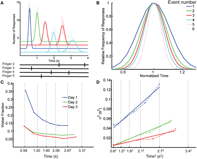
Figure 1. Spatiotemporal Pattern Reproduction task data. (A) Top panel: Distribution of response times for each key press (dotted lines), with Gaussian fits (solid lines), for a complex pattern from one subject; Bottom panel: the target pattern. Colors cyan, blue, red, and green, correspond to fingers 2 (index) through 5 (pinky). A systematic anticipation is noticeable at the longer responses in this subject. Although some subjects tended to produce early responses and others late, across subjects there was a tendency to anticipate the target time, particularly at the last responses in the pattern. On the last day of training the difference between the response time and target time at the first element in the pattern was (mean ± SD) 25 ± 75 ms (p = 0.26), whereas for the last element it was −230 ± 320 ms (p = 0.03). The spatial error rate (trials with incorrect finger presses) decreased rapidly over the first few blocks: in the first block, on average, 33% of the trials had a spatial error; this fell to 8% in the second block, and 0.9% by the last block (12). (B) Overlaid normalized Gaussian fits from (A). Each distribution has the x axis divided by its mean and their y values divided by their peak value. Dotted lines correspond to the second response of a given finger. (C) Weber fraction (=coefficient of variation) as a function of mean response time. Same subject, all 3 days. Vertical dotted lines indicate the target times. (D) Variance as a function of mean response time squared (dashed lines), and linear fits according to the generalized Weber’s law (Eq. 1, solid lines).
Our first observation is that the scalar property – the basic form of Weber’s law – is violated when subjects are timing spatiotemporal patterns. That is, the SD of the response time along the spatiotemporal pattern is not proportional to the mean response time, as demonstrated by plotting the normalized fits to the response distributions of the consecutive responses (Figure 1B). Figure 1C plots the CV of each response as a function of its time in the pattern for the same subject on each day, revealing a clear decrease in CV over time. Across the 12 subjects, on any given day, there was a significant decrease in the CV as revealed by a significant negative slope in relation to absolute time for all 3 days (p < 0.007).
This result indicates that the standard version of Weber’s law does not account for the changes in precision as a function of absolute time. The generalized version of Weber’s law (see Materials and Methods), however, robustly captured the relationship between precision and time of the response (Figure 1D). To provide a direct comparison for the generalized Weber fit, we also fit an equation where variance changes linearly with T instead of T2 (see Materials and Methods; Ivry and Hazeltine, 1995). Although both fits were quite good, the goodness of fit using Weber’s generalized law, as measured by the determination coefficient R2 between the fit and the data, was significantly better (mean R2 of 0.907 and 0.867, respectively; p = 0.0002 two-tailed paired t-test after Fisher transformation). It is also worth noting that for all 3 days the residuals were significantly smaller with the generalized Weber fit compared to a standard Weber fit (p < 0.001).
To the best of our knowledge these results are the first to show that “standard” Weber’s law does not hold for the timing of consecutively produced intervals. Yet, this result is consistent with previous results demonstrating violations in Weber’s law for individual intervals (Getty, 1975; Ivry and Hazeltine, 1995; Merchant et al., 2008; Lewis and Miall, 2009).
Learning Alters both Sources of Variance
Because timing in the STPR task was well accounted for by the generalized Weber’s law, we next examined how learning affected the time-dependent and time-independent variance sources. Figure 2A shows the learning curves for each of the 12 subjects across 3 days (four blocks of 20 trials each day). We defined performance as the error (RMS) between the response time and target times of each event. Learning of spatiotemporal patterns was observed for 8 out of the 12 subjects (see Materials and Methods).
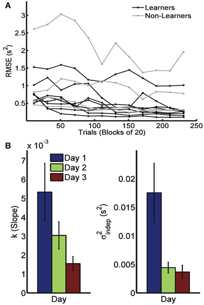
Figure 2. Learning in the spatiotemporal pattern reproduction task. (A) Learning curves. Performance of all subjects over 3 days of training. RMSE: root-mean-square error between response times and target times, averaged in blocks of 20 trials. Statistically significant learners are in black, non-learners in gray. Some subjects classified as non-learners had very low RMSE values, but did not exhibit any significant improvement in performance from the first to last block, and were thus classified as “non-learners” (see Materials and Methods). (B) Mean slope k and mean intercept  across the 3-days of training. Error bars represent the SEM. There was a significant decrease in both k and
  across training days (p = 0.013 and 0.011, respectively).
In order to determine how, and if, the parameters k and  change with learning we fit Weber’s generalized law to the data of each of the learners on each of the 3-days of training. We found that slope k and intercept
  both changed with learning (one-way, repeated-measures ANOVA; k: F2,6 = 6.04, p = 0.013;
  : F2,6 = 6.29, p = 0.011).
Experiment 2: Resetting versus Continuous Timing
An important question regarding the timing of patterns in which multiple responses are produced within a trial, is whether the internal timer is reset or not at each new interval during the production of the pattern. To examine this issue we trained 10 subjects in the TPR task (i.e., a purely temporal version of the previous task) in which every subject had to learn two different patterns: one periodic (six consecutive, equal intervals of 500 ms) and the other complex (a non-periodic pattern composed of six consecutive random intervals in the range 200–800 ms). The use of a purely temporal task as opposed to the spatiotemporal task used in Experiment 1 was important to rule out any potential variance generated by the spatial component (i.e., switching fingers).
The two contrasting hypotheses we tested are depicted in Figure 3. Under “Reset Timing” the timing of consecutive intervals is done independently, and thus the variance of the response time at each next event in the pattern adds to the accumulated variance from the previous responses (based on the result above, and those of others, we are assuming that the timing of any given interval is governed by Weber’s generalized law). In the case of a perfectly periodic pattern, this leads to a characteristic sublinear behavior when plotting the variance versus a time squared horizontal axis; for a complex pattern, in the reset mode the variance depends on the particular intervals of a pattern (see Materials and Methods for details). On the contrary, under “Continuous Timing,” for either periodic or complex patterns, the temporal pattern is processed in absolute time from its onset. Thus the variance at every event when timed from the onset of the pattern should follow the generalized form of Weber’s law, that is a straight line in a variance × time squared plot. These two qualitatively different behaviors of the variance can be tested by comparing the fit of the two models to the experimental data. We examined timing in both a periodic and complex task because we hypothesized that reset timing might be more likely to be used during periodic patterns.
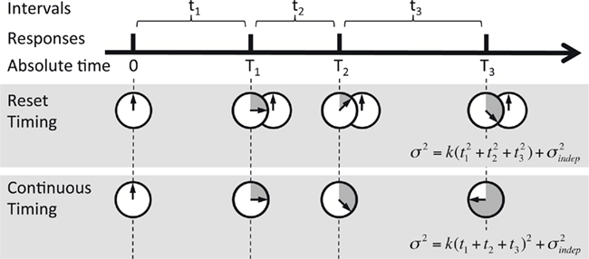
Figure 3. Reset versus continuous timing. Timing of a temporal pattern (thick black line) could be achieved by timing every interval tn in isolation and resetting the timer at each response (Reset timing), or by timing continuously in absolute time T since the beginning of the pattern (Continuous timing). The predicted variance at every point in the sequence is different, since in Reset timing the variance at each new response adds to the previous variance, whereas in Continuous timing the variance is a function of absolute time squared (note that T3 = t1 + t2 + t3).
In Figure 4A we show the experimental data from one subject after fitting the reset and continuous equations. The predicted variance under the Resetting hypothesis is decelerating, a trait not observed in the experimental data. The Continuous timing fit appears to better account for the variance in both the periodic and the complex pattern. To quantify this, we performed a repeated-measures two-way ANOVA with factors Model (Continuous versus Reset) and Training Day (1 through 5) on the Pearson correlation coefficient R (Fisher-transformed) between each model’s prediction and the experimental data (see Materials and Methods). The difference between Continuous and Reset models was significant for both the periodic and the complex patterns, with the Continuous producing a better fit than the Reset (periodic: mean R2 = 0.934 for the Continuous, mean R2 = 0.876 for the Reset, F1,9 = 49.9, p < 10−4; complex: mean R2 = 0.891 for the Continuous, mean R2 = 0.859 for the Reset, F1,9 = 11.2, p = 0.009; Figure 4B). There was no effect of training (periodic: F4,36 = 1.2, p = 0.31; complex: F4,36 = 1.0, p = 0.41) or interaction (periodic: F4,36 = 1.3, p = 0.28; complex: F4,36 = 0.4, p = 0.78), suggesting that the quality of the fits did not change with training.
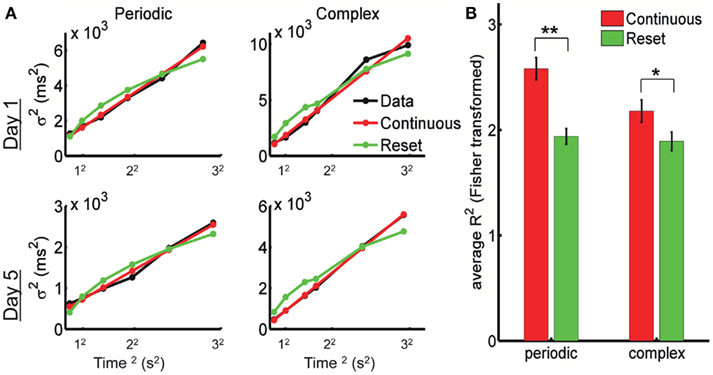
Figure 4. The psychophysical data is best fit by continuous timing. (A) Example of fits for Reset and Continuous timing from one subject: variance as a function of mean response time squared. Left column: periodic pattern; right column: complex pattern. Top row: training day 1; bottom row: training day 5. (B) Goodness of fit for Reset and Continuous: average R2 after Fisher transformation with SE bars. (**) p < 0.0001, (*) p = 0.009.
We also performed this same analysis with the spatiotemporal data in Experiments 1, with similar results. The Continuous model produced significantly better fits than the Reset model (mean R2 = 0.907 and 0.869, respectively; p = 0.01). This result suggests that the mechanism for timing consecutive intervals in a sequence does not change because of the presence of a spatial component. And interestingly, contrary to our expectations there is no significant difference between the quality of the Continuous for the temporal and spatiotemporal tasks (p = 0.61). Additionally, we verified that as in Experiment 1, the variance data was best fit by the generalized Weber equation. For the periodic patterns, the mean R2 was 0.934 and 0.878 for the generalized Weber (Eq. 1) and linear with T equation (Eq. 2), respectively (p < 10−5). For the complex patterns, the same mean R2 values were 0.891 and 0.854 (p = 10−4). The learning analysis for the data from Experiment 2 showed a very similar decreasing behavior of k and  as a function of training day, for both the periodic and the complex patterns.
Although these results suggest the Reset Timing should be rejected for both the periodic and the complex patterns and both the spatiotemporal and purely temporal tasks, it is interesting to note that the variance of the responses were consistently smaller for the periodic patterns (Figure 5). For example, although the target time of the last event of both the periodic and complex patterns was the same for all subjects and patterns (3 s), the variance was approximately double in the complex condition (both on Day 1 and 5). These observations suggest different modes or mechanisms of timing in the periodic and complex tasks (see Discussion).
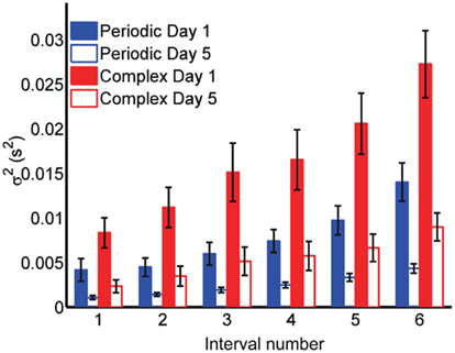
Figure 5. Variance is smaller for periodic patterns. Mean variance at each response for the first and last days of training. Although both periodic and complex patterns had the same total duration (3 s), the variance of the response times at the last response is smaller for the periodic pattern.
Model: Population Clock Based on Recurrent Network Dynamics Can Reproduce Timed Patterns
A number of previous models have proposed that the brain’s ability to tell time derives from the properties of neural oscillators operating in a clock-like fashion, through accumulation/integration of pulses emitted by a pacemaker. However, few studies have proposed detailed explanations of how these models account for the generation of multiple complex spatiotemporal patterns of the type studied in Experiment 1.
An alternate hypothesis to clock models suggest that timing emerges from the internal dynamics of recurrently connected neural networks, and that time is inherently encoded in the evolving activity pattern of the network – a population clock (Buonomano and Mauk, 1994; Buonomano and Laje, 2010). Here we focus on a population clock model that is well suited to account for the timing of complex spatiotemporal patterns, and is consistent with the results presented above suggesting that timing of patterns does not rely on a reset strategy. Since our psychophysical results above show that both spatiotemporal and temporal patterns are better accounted for by Continuous timing, in this section we focused on the more general problem of spatiotemporal pattern generation.
We implemented a population clock model in the form of a firing-rate recurrent neural network model (Buonomano and Laje, 2010). The network, displayed in Figure 6A, is composed of 1800 sparsely connected units, each with a time constant of 10 ms (see Materials and Methods). As shown in Figure 6B, a brief input can trigger a complex spatiotemporal pattern of activity within the recurrent network; and this pattern can be used to generate multiple, complex spatiotemporal output patterns several seconds in duration. Different output patterns can be triggered by different brief input stimuli. The results shown are from a network with three inputs and four outputs (each output represents a finger). Input 1 (tonic) sets the network outputs in a state of low-level activity, while Inputs 2 and 3 (pulsed) act as “go” signals for patterns 1 and 2, respectively. The four output units feedback to the network, and the corresponding four sets of output weights are subject to training with the FORCE learning algorithm (Sussillo and Abbott, 2009). The network is trained to reproduce the desired target pattern every time the corresponding ”go” signal is activated. In this scenario learning takes place by adjusting the weights on to the readout units. To simulate the responses used in our STPR task (discrete, pulse-like finger movements) the target response is simulated as a smooth but rapidly ascending and descending waveform.
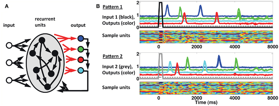
Figure 6. Population clock model based on recurrent network dynamics. (A) Network architecture. The four output units are meant to represent the four fingers. Only the readout connections (depicted in red) are subject to training. (B) Reproduction of two complex spatiotemporal patterns (each with three different runs overlaid) after adjusting the weights of the recurrent units onto the readout units. Output traces are shifted vertically for visual clarity. Each pattern is triggered by a brief activation (100 ms) of the corresponding input unit at t = 0 (black thick trace, Pattern 1; gray thick trace, Pattern 2). The dashed black trace represents a (third) constant input to the recurrent network. Colored rasters represent a subset (20) of the recurrent units. In these units activity ranges from −1 (blue) to 1 (red).
Our numerical simulations reveal that the variance signature exhibited by the model is strongly dependent on the parameters of the model (including the synaptic strength factor g, and the strength of the feedback, see Rajan et al., 2010). In the simulation presented here on average variance increased approximately linearly with T2 (with a large degree of variation between simulations). However, variance values were much smaller than those observed experimentally: a Weber fraction of around 1% (compare with the experimental Weber fraction on the order of 10–30% in Figure 1C). It is well known that the dynamics of recurrent networks is highly complex and prone to chaotic activity (Sompolinsky et al., 1988; Jaeger and Haas, 2004; Rajan et al., 2010), while outside the scope of the current study it is clear that it will be necessary to better understand the dynamics of these systems to determine if they can quantitatively account for the experimentally observed variance signature (see Discussion).
Qualitatively the population clock framework shown in Figure 6 elegantly accounts for both the spatial and temporal aspects of complex spatiotemporal patterns. That is, the spatial pattern, the timing, and the order of the fingers are all encoded in a multiplexed fashion in the recurrent network plus the readout. Furthermore, the model is most consistent with “continuous” timing, and thus with the experimental data. Specifically, while a feedback loop from the output units to the recurrent network could be used to implement reset timing, such a reset signal would necessarily bring the network to the same state every time that finger was used during a pattern. Consider the production of an aperiodic temporal pattern, and now suppose that the output pulse “resets” the network state through the feedback loop. Resetting to the same state would trigger the same neural trajectory, making the same output fire again leading to a periodic loop. Although the same motor response can be triggered by many different internal states (a many-to-one mapping), every time that motor response is generated it would erase the previous history of the recurrent network through the reset command. However, a reset strategy could potentially be implemented if additional assumptions were incorporated, such as buffers that kept track of the ordinal position of each response. Lastly it should be pointed out that, since recurrent networks seem to exhibit a range of different variance signatures depending on model parameters, it is theoretically possible that in some regimes the model could emulate a reset timing variance signature without actually being reset.
Discussion
Weber versus Generalized Weber
The great majority of timing studies that have quantified changes in temporal precision as a function of the interval being timed have examined each interval independently – that is, timing of 500 and 1000 ms intervals would be obtained on separate trials (for reviews see, Gibbon et al., 1997; Ivry and Spencer, 2004; Mauk and Buonomano, 2004; Buhusi and Meck, 2005; Grondin, 2010). Here we examined scaling of temporal precision during a sequential reproduction task in which subjects were required to time different absolute temporal intervals within the same trials. Consistent with a number of previous studies (Getty, 1975; Ivry and Hazeltine, 1995; Hinton and Rao, 2004; Bizo et al., 2006; Merchant et al., 2008; Lewis and Miall, 2009), we established that in consecutive timing, precision also does not follow the standard version of Weber’s law; in other words, the Weber fraction calculated as the CV decreased with increasing intervals (Figure 1).
Consistent, again, with a number of previous studies we found that the variance of consecutively timed motor responses were well accounted for by the generalized version of Weber’s law – specifically, that variance increases with absolute time squared (Getty, 1975; Ivry and Hazeltine, 1995; Bizo et al., 2006; Merchant et al., 2008). Weber’s law is, of course, a specific instance of the generalized law in which the intercept (the time-independent variance) is equal to zero. Thus previous results conforming to Weber’s law are likely to represent instances in which the non-temporal variance is relatively small compared to the temporal variance. Indeed, most of the studies supporting Weber’s law have not explicitly examined whether the reported data would not be significantly better fit by Weber’s generalized law.
Effects of Learning
The fact that the data was very well fit by Weber’s generalized law allowed us to ask whether learning of spatiotemporal patterns altered the time-dependent and/or independent sources of variance. Traditionally, the time-dependent portion of the variance is interpreted as reflecting the properties of a clock or timing device. The time-independent variance is often taken to reflect the noise in the motor response or “internal” noise that non-specifically alters sensory and/or motor aspects of any psychophysical task. It is not immediately clear which of the potential sources of variance would be expected to underlie the improved performance that occurs with practice. We observed that both  and the slope k (which approximates the traditional Weber fraction at long intervals) change over the course of learning (Figure 2). Visually,
  seemed to change and asymptote more rapidly thank k (Figure 2), this was not statistically significant however. Nevertheless, in future experiments it will be of interest to determine if both sources of variance can change independently during learning. We interpret
  as reflecting an amalgam of internal noise sources including both motor and attentional factors, and speculate that some of the improvements in
  are likely to reflect attentional components that would generalize across different temporal patterns.
As mentioned, the coefficient k of the time-dependent term is often interpreted as reflecting the property of an internal clock; more specifically, as capturing the variation in the generation of pulses of a hypothetical pacemaker. Within this framework one might interpret the improvement in k as a decrease in the variability of a pacemaker. We have previously argued that motor (and sensory) timing does not rely on an internal clock, but rather as exemplified in Figure 6, on the dynamics of recurrently connected neural networks (Mauk and Buonomano, 2004; Buonomano and Laje, 2010). Within this framework we would interpret the decrease in k as reflecting less cross-trial variability in the neural trajectory (see below). However, it remains far from clear what the decrease in k truly reflects at the neural level.
Reset versus Continuous Timing
The use of consecutively timed responses during the STPR task, as opposed to the timing of independent intervals, raises an important question: when timing multiple consecutive intervals does the internal timer – whatever its nature – operate continuously throughout the entire pattern, or does it “reset” at each event (Figure 3)? To use a stopwatch analogy, if you need to time two consecutive intervals, one of 1 s and the second of 1.5 s, do you start a stopwatch at t = 0 ms, generate a response at 1 s, then wait until it hits 2.5 s and generate another, or do you reset/restart the stopwatch at 1 s, and generate a second response at 1.5 s?
This question relates to previous studies that have examined the effects of subdividing on timing. Specifically, to generate a multi-second response, it is typically reported that “counting” (which generates subintervals), improves precision (Fetterman and Killeen, 1990; Hinton and Rao, 2004; Hinton et al., 2004; Grondin and Killeen, 2009). One interpretation of this result is that since timing precision increases as a function of absolute time squared T2, total variance is less if the total interval T is subdivided into t1 + t2, because  In other words, counting may be superior because in essence the internal timer is being reset during each subinterval.
To address the question of whether the internal timer is reset during a pattern we examined whether temporal precision is best fit by continuous or reset assumptions during the reproduction of both periodic and complex temporal patterns. Our results reveal that both fits were actually pretty good (R2 > 0.86), and that the difference between both models can be surprisingly subtle and potentially easily missed. Nevertheless, our findings clearly indicate that for both periodic and complex stimuli the fits using the continuous model produced significantly smaller residuals. These results suggest that the neural mechanisms underlying timing appear to accumulate variance over the course of a pattern in a manner consistent with continuous operation of a timing device. We initially expected that there may be a difference between periodic and complex patterns, specifically, that precision during periodic patterns would more likely be consistent with a reset mechanism. However, this expectation was not supported, as the continuous fits were significantly better for both the periodic and complex patterns.
Nevertheless, consistent with studies showing that counting, and thus presumably periodic subdividing, improves performance, we did observe a significant decrease in total variance of the last event, which was the same for the periodic and complex patterns (3 s). Interestingly there was also difference for the first event between both tasks (500 ms in the periodic patterns, and on average 598 ms in the complex patterns; Figure 5). It is noteworthy that by the end of training, the absolute precision of a few subjects was comparable in the periodic and complex tasks, raising the possibility that comparable precision can be achieved in periodic and complex patterns.
These results raise somewhat of a conundrum: timing of a 3-s response is indeed better if the previous five responses were equally spaced compared to an aperiodic pattern; however, the improvement does not appear to be a result of resetting during the periodic task. Are different circuits responsible for the periodic and complex timing? Is periodic timing less flexible, thus allowing for better precision? We cannot speak directly to these questions here; however, in the sensory domain it has been suggested that there may be different neural circuits for periodic and non-periodic timing (Grube et al., 2010; Teki et al., 2011). Still, it remains a possibility that given the relatively small, but significant, difference in the quality of the fits between the reset and continuous timing equations, we were not able to pick out subtle differences between them. It is also possible that, since our subjects were reproducing both patterns in alternation, they were nudged toward using similar “continuous” strategies. Finally, less precise timing in complex conditions might simply reflect non-specific factors relating to the task requirements, e.g., increase attentional and memory load.
Models of Timing
A critical challenge to any model of timing is to provide a mechanistic description of its postulated underpinning in biologically plausible terms. A number of models have proposed that the brain’s ability to tell time derives from the properties of neural oscillators operating in a clock-like fashion, yielding an explicit, linear metric of time (Creelman, 1962; Treisman, 1963). Others have proposed a population of neural elements oscillating at different frequencies, with a readout mechanism that detects specific beats or coincidental activity at specific points in time (Miall, 1989; Matell and Meck, 2004). Still others propose that time might be directly encoded in the activity of neural elements with differing time constants of some cellular or synaptic property (for a review see, Mauk and Buonomano, 2004). As a general rule, many models of timing have focused primarily on the timing of single isolated intervals, as opposed to the generation of multiple complex spatiotemporal patterns as examined here. Indeed, it is not immediately clear how the clock models based on the integration of events from a pacemaker can account for generating different temporal patterns in a flexible fashion. For this reason, here we have focused on network models, which in our opinion can elegantly capture the spatial, timing, and order components of complex motor tasks.
In addition to being implemented at the levels of neurons, any model must of course also account for the behavioral and psychophysical data. Indeed, one of the strengths of psychophysical studies is to test and constrain mechanistic models of timing. The neural mechanism of timing remains debated, but it is increasingly clear that there are likely multiple areas involved, and that different neural mechanisms may underlie timing on the scale of milliseconds and seconds (for reviews see, Buonomano and Karmarkar, 2002; Mauk and Buonomano, 2004; Buhusi and Meck, 2005; Ivry and Schlerf, 2008; van Wassenhove, 2009; Grondin, 2010). One biologically based model of timing suggests that dynamic changes in the population of active neurons encode time. This model, first proposed in the context of the cerebellum (Buonomano and Mauk, 1994; Mauk and Donegan, 1997; Medina et al., 2000), and later in recurrent excitatory circuits (Buonomano and Merzenich, 1995; Buonomano and Laje, 2010) has been referred to as a population clock (Buonomano and Karmarkar, 2002). In the motor domain, any time-varying neural activity requires either continuous input or internally generated changes in network state. This class of models is most consistent with Continuous timing (see Results). Specifically, since timing relies on setting a particular neural trajectory in motion, different points in time (as well as the ordinal position and the appropriate finger) are coded in relation to the initial state at t = 0 (Figure 6) – resetting the network, in contrast, can erase information about ordinal position and finger pattern embedded in the recurrent network.
In vivo electrophysiological studies have lent support to the notion of a population clock, including reports of neurons that fire at select time intervals or in a complex aperiodic manner (Hahnloser et al., 2002; Matell et al., 2003; Jin et al., 2009; Long et al., 2010; Itskov et al., 2011). In the experimental and theoretical studies the temporal code of a population clock can take various forms: First, time might be encoded in a feed-forward chain, where each neuron essentially responds at one time point (Hahnloser et al., 2002; Buonomano, 2005; Liu and Buonomano, 2009; Fiete et al., 2010; Long et al., 2010; Itskov et al., 2011); Second, the code can be high dimensional, where at one point in time is encoded in the active population response of many neurons, and each neuron can fire at multiple time points (Medina and Mauk, 1999; Medina et al., 2000; Lebedev et al., 2008; Jin et al., 2009; Buonomano and Laje, 2010). Indeed, some of these studies have shown that a linear classifier (readout unit) can be used to decode time based on the profiles of the experimentally recorded neurons, thus effectively implementing a population clock (Lebedev et al., 2008; Jin et al., 2009; Crowe et al., 2010).
While experimental data showing that different neurons or populations of neurons respond at different points in time supports the notion that time is encoded in the dynamics of neural network – in the neural trajectories – at the theoretical level it has been challenging to generate recurrent excitatory networks capable of producing reliable (“non-chaotic”) patterns. While recent progress has been made in both physiological learning rules that may account for the formation of neural trajectories (Buonomano, 2005; Liu and Buonomano, 2009; Fiete et al., 2010) and the circuit architecture that might support them (Jaeger and Haas, 2004; Sussillo and Abbott, 2009; Itskov et al., 2011), these models have not explicitly captured the variance characteristics (Weber’s generalized law) observed psychophysically. This holds true for the model presented in Figure 6 (which tends to exhibit very little variance; or, as the noise is increased, variance that scales too rapidly). Thus, while this class of models is consistent with the notion that the internal timer does not reset during the production of patterns, future models must accurately capture the known relationship between precision and absolute time.
Conflict of Interest Statement
The authors declare that the research was conducted in the absence of any commercial or financial relationships that could be construed as a potential conflict of interest.
Acknowledgments
We would like to acknowledge the European project COST ISCH Action TD0904 TIMELY, the Pew Charitable Trusts, and CONICET (Argentina).
References
Allan, L. G., and Gibbon, J. (1991). Human bisection at the geometric mean. Learn. Motiv. 22, 39–58.
Bizo, L. A., Chu, J. Y., Sanabria, F., and Killeen, P. R. (2006). The failure of Weber’s law in time perception and production. Behav. Processes 71, 201–210.
Buhusi, C. V., and Meck, W. H. (2005). What makes us tick? Functional and neural mechanisms of interval timing. Nat. Rev. Neurosci. 6, 755–765.
Buonomano, D. V. (2005). A learning rule for the emergence of stable dynamics and timing in recurrent networks. J. Neurophysiol. 94, 2275–2283.
Buonomano, D. V., and Laje, R. (2010). Population clocks: motor timing with neural dynamics. Trends Cogn. Sci. (Regul. Ed.) 14, 520–527.
Buonomano, D. V., and Mauk, M. D. (1994). Neural network model of the cerebellum: temporal discrimination and the timing of motor responses. Neural Comput. 6, 38–55.
Buonomano, D. V., and Merzenich, M. M. (1995). Temporal information transformed into a spatial code by a neural network with realistic properties. Science 267, 1028–1030.
Carr, C. E. (1993). Processing of temporal information in the brain. Annu. Rev. Neurosci. 16, 223–243.
Church, R. M., Meck, W. H., and Gibbon, J. (1994). Application of scalar timing theory to individual trials. J. Exp. Psychol. Anim. Behav. Process. 20, 135–155.
Crowe, D. A., Averbeck, B. B., and Chafee, M. V. (2010). Rapid sequences of population activity patterns dynamically encode task-critical spatial information in parietal cortex. J. Neurosci. 30, 11640–11653.
Fetterman, J. G., and Killeen, P. R. (1990). A componential analysis of pacemaker-counter timing systems. J. Exp. Psychol. Hum. Percept. Perform. 16, 766–780.
Fiete, I. R., Senn, W., Wang, C. Z. H., and Hahnloser, R. H. R. (2010). Spike-time-dependent plasticity and heterosynaptic competition organize networks to produce long scale-free sequences of neural activity. Neuron 65, 563–576.
Getty, D. J. (1975). Discrimination of short temporal intervals: a comparison of two models. Percept. Psychophys. 18, 1–8.
Gibbon, J. (1977). Scalar expectancy theory and Weber’s law in animal timing. Psychol. Rev. 84, 279–325.
Gibbon, J., Malapani, C., Dale, C. L., and Gallistel, C. R. (1997). Toward a neurobiology of temporal cognition: advances and challenges. Curr. Opin. Neurobiol. 7, 170–184.
Grondin, S. (2010). Timing and time perception: a review of recent behavioral and neuroscience findings and theoretical directions. Atten. Percept. Psychophys. 72, 561–582.
Grondin, S., and Killeen, P. R. (2009). Tracking time with song and count: different Weber functions for musicians and nonmusicians. Atten. Percept. Psychophys. 71, 1649–1654.
Grube, M., Cooper, F. E., Chinnery, P. F., and Griffiths, T. D. (2010). Dissociation of duration-based and beat-based auditory timing in cerebellar degeneration. Proc. Natl. Acad. Sci. U.S.A. 107, 11597–11601.
Hahnloser, R. H. R., Kozhevnikov, A. A., and Fee, M. S. (2002). An ultra-sparse code underlies the generation of neural sequence in a songbird. Nature 419, 65–70.
Hinton, S. C., Harrington, D. L., Binder, J. R., Durgerian, S., and Rao, S. M. (2004). Neural systems supporting timing and chronometric counting: an FMRI study. Cogn. Brain Res. 21, 183–192.
Hinton, S. C., and Rao, S. M. (2004). “One-thousand one… one-thousand two…”: chronometric counting violates the scalar property in interval timing. Psychon. Bull. Rev. 11, 24–30.
Itskov, V., Curto, C., Pastalkova, E., and Buzsáki, G. (2011). Cell assembly sequences arising from spike threshold adaptation keep track of time in the hippocampus. J. Neurosci. 31, 2828–2834.
Ivry, R. B., and Hazeltine, R. E. (1995). Perception and production of temporal intervals across a range of durations – evidence for a common timing mechanism. J. Exp. Psychol. Hum. Percept. Perform. 21, 3–18.
Ivry, R. B., and Schlerf, J. E. (2008). Dedicated and intrinsic models of time perception. Trends Cogn. Sci. (Regul. Ed.) 12, 273–280.
Ivry, R. B., and Spencer, R. M. C. (2004). The neural representation of time. Curr. Opin. Neurobiol. 14, 225–232.
Jaeger, H., and Haas, H. (2004). Harnessing nonlinearity: predicting chaotic systems and saving energy in wireless communication. Science 304, 78–80.
Jazayeri, M., and Shadlen, M. N. (2010). Temporal context calibrates interval timing. Nat. Neurosci. 13, 1020–1026.
Jin, D. Z., Fujii, N., and Graybiel, A. M. (2009). Neural representation of time in cortico-basal ganglia circuits. Proc. Natl. Acad. Sci. U.S.A. 106, 19156–19161.
King, D. P., and Takahashi, J. S. (2000). Molecular genetics of circadian rhythms in mammals. Annu. Rev. Neurosci. 23, 713–742.
Lebedev, M. A., O’Doherty, J. E., and Nicolelis, M. A. L. (2008). Decoding of temporal intervals from cortical ensemble activity. J. Neurophysiol. 99, 166–186.
Lewis, P. A., and Miall, R. C. (2009). The precision of temporal judgement: milliseconds, many minutes, and beyond. Philos. Trans. R. Soc. B Biol. Sci. 364, 1897–1905.
Lewis, P. A., Miall, R. C., Daan, S., and Kacelnik, A. (2003). Interval timing in mice does not rely upon the circadian pacemaker. Neurosci. Lett. 348, 131–134.
Liu, J. K., and Buonomano, D. V. (2009). Embedding multiple trajectories in simulated recurrent neural networks in a self-organizing manner. J. Neurosci. 29, 13172–13181.
Long, M. A., Jin, D. Z., and Fee, M. S. (2010). Support for a synaptic chain model of neuronal sequence generation. Nature 468, 394–399.
Matell, M. S., and Meck, W. H. (2004). Cortico-striatal circuits and interval timing: coincidence detection of oscillatory processes. Cogn. Brain Res. 21, 139–170.
Matell, M. S., Meck, W. H., and Nicolelis, M. A. (2003). Interval timing and the encoding of signal duration by ensembles of cortical and striatal neurons. Behav. Neurosci. 117, 760–773.
Mauk, M. D., and Buonomano, D. V. (2004). The neural basis of temporal processing. Annu. Rev. Neurosci. 27, 307–340.
Mauk, M. D., and Donegan, N. H. (1997). A model of Pavlovian eyelid conditioning based on the synaptic organization of the cerebellum. Learn. Mem. 3, 130–158.
Meck, W. H., and Church, R. M. (1987). Cholinergic modulation of the content of temporal memory. Behav. Neurosci. 101, 457–464.
Medina, J. F., Garcia, K. S., Nores, W. L., Taylor, N. M., and Mauk, M. D. (2000). Timing mechanisms in the cerebellum: testing predictions of a large-scale computer simulation. J. Neurosci. 20, 5516–5525.
Medina, J. F., and Mauk, M. D. (1999). Simulations of cerebellar motor learning: computational analysis of plasticity at the mossy fiber to deep nucleus synapse. J. Neurosci. 19, 7140–7151.
Merchant, H., Zarco, W., and Prado, L. (2008). Do we have a common mechanism for measuring time in the hundreds of millisecond range? evidence from multiple-interval timing tasks. J. Neurophysiol. 99, 939–949.
Miall, C. (1989). The storage of time intervals using oscillating neurons. Neural Comput. 1, 359–371.
Nissen, M. J., and Bullemer, P. (1987). Attentional requirements of learning: evidence from performance measures. Cogn. Psychol. 19, 1–32.
Panda, S., Hogenesch, J. B., and Kay, S. A. (2002). Circadian rhythms from flies to human. Nature 417, 329–335.
Rajan, K., Abbott, L. F., and Sompolinsky, H. (2010). Stimulus-dependent suppression of chaos in recurrent neural networks. Phys. Rev. E Stat. Nonlin. Soft Matter Phys. 82, 011903.
Shin, J. C., and Ivry, R. B. (2002). Concurrent learning of temporal and spatial sequences. J. Exp. Psychol. Learn. Mem. Cogn. 28, 445–457.
Sompolinsky, H., Crisanti, A., and Sommers, H. J. (1988). Chaos in random neural networks. Phys. Rev. Lett. 61, 259–262.
Sussillo, D., and Abbott, L. F. (2009). Generating coherent patterns of activity from chaotic neural networks. Neuron 63, 544–557.
Teki, S., Grube, M., Kumar, S., and Griffiths, T. D. (2011). Distinct neural substrates of duration-based and beat-based auditory timing. J. Neurosci. 31, 3805–3812.
Treisman, M. (1963). Temporal discrimination and the indifference interval: implications for a model of the ‘internal clock.’ Psychol. Monogr. 77, 1–31.
Keywords: timing, temporal processing, time estimation and production, human psychophysics, recurrent networks, neural dynamics, computational modeling
Citation: Laje R, Cheng K and Buonomano DV (2011) Learning of temporal motor patterns: an analysis of continuous versus reset timing. Front. Integr. Neurosci. 5:61. doi: 10.3389/fnint.2011.00061
Received: 29 June 2011; Paper pending published: 09 July 2011;
Accepted: 25 September 2011; Published online: 13 October 2011.
Edited by:
Warren H. Meck, Duke University, USACopyright: © 2011 Laje, Cheng and Buonomano. This is an open-access article subject to a non-exclusive license between the authors and Frontiers Media SA, which permits use, distribution and reproduction in other forums, provided the original authors and source are credited and other Frontiers conditions are complied with.
*Correspondence: Dean V. Buonomano, Departments of Neurobiology and Psychology, University of California, 695 Young Drive, Gonda – Room 1320, Los Angeles, CA 90095-1761, USA. e-mail: dbuono@ucla.edu