


Abstract
Myocardial deformation is a key to clinical decision-making. Feature-tracking cardiovascular magnetic resonance (FT-CMR) provides quantification of motion and strain using standard steady-state in free-precession (SSFP) imaging, which is part of a routine CMR left ventricular (LV) study protocol. An accepted definition of a normal range is essential if this technique is to enter the clinical arena.
One hundred healthy individuals, with 10 men and women in each of 5 age deciles from 20 to 70 years, without a history of cardiovascular disease, diabetes, renal impairment, or family history of cardiovascular disease, and with a normal stress echocardiogram, underwent FT-CMR assessment of LV myocardial strain and strain rate using SSFP cines.
Peak systolic longitudinal strain (Ell) was −21.3 ± 4.8%, peak systolic circumferential strain (Ecc) was −26.1 ± 3.8%, and peak systolic radial strain (Err) was 39.8 ± 8.3%. On Bland–Altman analyses, peak systolic Ecc had the best inter-observer agreement (bias 0.63 ± 1.29% and 95% CI −1.90 to 3.16) and peak systolic Err the least inter-observer agreement (bias 0.13 ± 6.41 and 95% CI −12.44 to 12.71). There was an increase in the magnitude of peak systolic Ecc with advancing age, which was greatest in subjects over the age of 50 years (R2 = 0.11, P = 0.003). There were significant gender differences (P < 0.001) in peak systolic Ell, with a greater magnitude of deformation in females (−22.7%) than in males (−19.3%).
Normal values for myocardial strain measurements using FT-CMR are provided. All circumferential and longitudinal based variables had excellent intra- and inter-observer variability.
Background
The assessment of left ventricular (LV) function is, arguably, the most important component of a cardiac imaging study. In routine clinical practice using either echocardiography or cardiovascular magnetic resonance (CMR), this consists of assessments of global systolic and diastolic function. It is well recognized, however, that global measures, such as left ventricular ejection fraction (LVEF), may not be sensitive enough to detect subtle changes in LV function, as is the case with incipient disease.1,2
Cardiac strain, a sensitive measure of deformation, is defined as the relative change in fibre length from end diastole. While measuring this in vivo would require a precise knowledge of the local fibre direction, clinical imaging modalities circumnavigate this by measuring strain in three principal directions (radial, circumferential, and longitudinal), relative to the central axis of the ventricle. Measurements of strain are becoming increasingly popular in both clinical and research environments. However, echocardiographic measurements obtained using tissue Doppler imaging3,4 are limited by noise interference and angle dependency.5 While speckle tracking has largely overcome these issues, it is often limited by image quality.6
CMR imaging combined with myocardial tagging is the reference-standard technique for the assessment of myocardial motion. Myocardial tags created by manipulating magnetisation act as fiducial markers that conform to the region of interest.7 A variety of techniques, such as harmonic phase analysis (HARP) or spatial modulation of magnetisation (SPAMM), can be used to quantify myocardial displacement, strain, and strain rate.8 These techniques have been validated for the assessment of regional wall motion in animals and humans.9 To date, however, myocardial tagging acquisition and its requisite post-processing analysis are largely confined to the research environment, not least because they are laborious and time consuming.
Feature-tracking CMR (FT-CMR) is a novel technique that allows quantification of motion and strain using a standard steady-state in free-precession (SSFP) sequence, which forms part of a routine LV study protocol. Whereas myocardial tagging provides a pan-myocardial assessment of deformation, FT-CMR is relatively crude, as it is limited to the assessment of myocardial edges. Nevertheless, FT-CMR, which has been validated against myocardial tagging using HARP10 and SPAMM,11 involves rapid acquisition and post-processing. We have quantified normal LV myocardial strain and strain rates in a large cohort of healthy adults with a wide age range.
Methods
Patient recruitment
One hundred subjects were recruited in a pre-determined, stratified fashion to provide 10 participants of each gender, representing each age decade from vicenarians to sexagenarians. Healthy control subjects were identified from an ongoing controlled prospective observational research study examining the effects of living kidney donation on cardiovascular structure and function (NCT01769924).12 Rigorous screening criteria were applied: a 10-year risk of a cardiovascular event of <20% as evaluated using the QRISK-2 index,13,14 normal exercise stress echocardiography, and normal haematology and biochemistry profiling. Exclusion criteria included: any history of cardiovascular disease, any history of diabetes or glucose intolerance, renal impairment, anaemia or atrial fibrillation, first-degree relative with a proved or potentially inheritable cardiac condition, or a history of premature coronary artery disease. Recruits with an office blood pressure >140 mmHg systolic or 90 mmHg diastolic had to have a 24-h ambulatory average of <135/85 mmHg to meet our inclusion criteria. However, in such individuals, office blood pressure was used in analyses, as not all recruits underwent ambulatory monitoring. Previous prescription of an anti-hypertensive medication was an exclusion criteria.
CMR acquisition
This was performed with a 1.5 Tesla scanner (Magnetom Avanto, Siemens, Erlangen, Germany), using a phased-array cardiac coil. A horizontal long-axis image and a short-axis LV stack from the atrioventricular ring to the LV apex were acquired using an SSFP (repetition time of 3.2 ms; echo time of 1.7 ms; flip angle of 60°; sequential 7 mm slices with a 3 mm interslice gap). There were 25 phases per cardiac cycle resulting in a mean temporal resolution of 40 ms.
Evaluation of LV dimensions, function, and mass
LV mass and LV end-diastolic (LVEDV) and end-systolic (LVESV) ventricular volumes were quantified using manual planimetry of the endocardial and epicardial borders from the short-axis stack, in accordance with validated methodologies15 using Argus software (Siemens, Erlangen, Germany). These were indexed to body surface area using the Mosteller formula.16
Feature tracking
FT-CMR was undertaken using the Diogenes FT-CMR software (TomTec Imaging Systems, Munich, Germany). The base was selected as the slice closest to the annulus without through plane distortion from the LV outflow tract. The horizontal long-axis SSFP was used to identify the true mid cavity at end diastole (equidistant between apex and ring), and the apical slice used was that closest to being equidistant between the apical tip and the mid cavity at end diastole. (Figure 1).
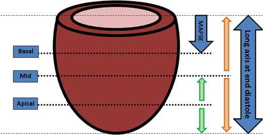
Methodology for slice selection for FT-CMR. A consistent methodology for slice selection is imperative as FT-CMR offers a greater choice of cines for post-processing compared with echocardiography or myocardial tagging, particularly as apical images can be tracked. The schematic demonstrates the optimal slices to select for FT-CMR. All slices are selected in end diastole. The mid slice should represent the mid cavity at end diastole (orange arrows). The apical slice is chosen as the midpoint between the mid slice and the apical tip of the LV (green arrows). The basal slice should be the distance of the mitral annular plane systolic excursion away from atrioventricular ring in end diastole (purple arrow) to prevent extra-ventricular structures distorting the analyses. These are the optimal positions for slices, but an advantage of FT-CMR is that it can be performed on the SSFP sequences which are part of a routine protocol. The slices that correspond closest to these positions should be selected for post-processing with FT-CMR. MAPSE: mitral annular plane systolic excursion.
Endocardial and epicardial borders were manually drawn in the end-diastolic frame (Figure 2). Papillary muscles were excluded from the endocardial contour. These were then automatically propagated (tracked) through the cardiac cycle by matching individual patterns that represent anatomical structures. These were identified by the method of maximum likelihood between the regions of interest of consecutive frames.17 The distance moved by individual points within the 2D matrix between frames permitted computation of displacement and strain. Their first order derivatives, velocity and strain rate, were calculated by the process of optical flow, i.e. the ratio between distance and the time interval between frames.18
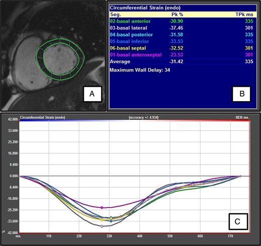
Feature-tracking CMR. (A) Endocardial and epicardial contours are traced in the end-diastole frame. (B) Peak systolic strain is given for each equiangular segment. The anterior segment is manually delineated starting at the anterior septum. The (global) peak systolic strain is not an average of the peak systolic strain for each segment, but a true instantaneous peak strain (derived from the average global strain at each time point). (C) A colour-coded plot of strain vs. time is shown for each segment. For segmental plots, only the peak systolic strain is marked. The average plot is the masked middle white line but this can be easily recognized as strain is plotted at each time point.
To minimize variability, user adjustments after the first attempt at tracking were kept to a minimum. However, as with any deformation technique, inaccuracies can arise, because the boundary between the trabecular and compact portions of the wall may shift as the blood spaces between the trabeculae close during systole, resulting in an artefactual, apparent inward motion of the endocardial contour. If this was deemed to be a significant problem, the cine was re-tracked with manual contouring using an end-systolic frame.
Horizontal long-axis cines were tracked to derive longitudinal displacement and strain, while short-axis cines were used to derive circumferential and radial displacements and strain. Separate endocardial and epicardial values were calculated for longitudinal and circumferential strain. Only one measure of strain was calculated in the radial direction, as this direction (myocardial thickening and thinning) is perpendicular to the endocardial and epicardial borders, so both contours are required to derive transmural radial strain.
Global peak systolic longitudinal (Ell), radial (Err), and circumferential (Ecc) strains; global peak systolic longitudinal (SRll), radial (SRrr), and circumferential (SRcc) strain rates; and global peak early diastolic longitudinal (DSRll), radial (DSRrr), and circumferential (DSRcc) strain rates were all derived. Segmental peak systolic circumferential strains (in accordance with the American Heart Association's 16-segment model) were also derived.
Reproducibility
For the assessment of inter-observer variability, a randomly generated set of 20 scans were tracked by two investigators (R.J.T. and W.E.M.). The same cine was assessed by each operator, who saved the results independently of the other, to provide a blinded assessment. Investigator 1 (R.J.T.) repeated this process 1 month later to assess intra-observer agreement.
Statistical analyses
Continuous variables are expressed as mean ± standard deviation (SD). Normality was tested using the Shapiro–Wilk test. Comparisons between segments were made using repeated-measures ANOVA. Independent sample t-tests were used to compare inter-gender differences. Curve fitting was performed to assess the relationship between strain and age. Linear regression analysis was used to explore the relationship between strain and baseline variables. Variables reaching a P-value of <0.10 were included in multivariable models. Agreement was tested by calculating mean bias and 95% limits of agreement (confidence intervals) from Bland–Altman analyses, coefficient of variation, and inter-class correlation coefficient (ICC). A P-value of <0.05 was considered statistically significant. Statistical analysis was performed using SPSS v21.0. (SPSS, Inc., Chicago, IL, USA).
Results
Baseline demographics
The baseline demographics of the entire cohort of 100 healthy individuals are shown in Table 1. They were normotensive (mean daytime ambulatory systolic blood pressure 123 ± 12 mmHg; mean daytime ambulatory diastolic blood pressure 73 ± 7 mmHg). Fasting total cholesterol was 5.0 ± 1.1 mmol/L, fasting total cholesterol/HDL ratio was 3.4 ± 1.0, and fasting glucose was 4.7 ± 0.4 mmol/L. Estimated glomerular filtration rate, using the modification by diet of renal disease equation, was >60 mL/min/1.73 m2 in all participants. All participants had a 10-year QRISK-2 score of ≤ 20%. Cardiac volumes, mass, and ejection fraction were within normal limits for all participants.15 There was an age-dependent effect on LVEF, LVESV, and LVEDV (P < 0.001 for all) (Figure 3).
Baseline characteristics
| Mean ± SD or n (%) | |
|---|---|
| Demographics | |
| Age | 44.5 ± 14.0 |
| Sex (Male) | 50 |
| Height (cm) | 170.0 ± 9.6 |
| Weight (kg) | 74.3 ± 12.4 |
| Body surface area (m2) | 1.85 ± 0.2 |
| Co-morbidities | |
| Smoker—Current | 8 |
| Smoker—Ex | 19 |
| Fasting total cholesterol (mmol/L) | 5.01 ± 1.1 |
| Fasting total cholesterol/HDL ratio | 3.4 ± 1.0 |
| Hypercholesterolaemia (%)a | 10 |
| Fasting glucose (mmol/L) | 4.7 ± 0.4 |
| eGFR > 60 mL/min/1.73 m2 | 100 |
| 10-year cardiovascular risk (%) | 3.6 (0.4–5.8) |
| Haemoglobin (g/dL) | 13.8 ± 1.3 |
| Haemodynamic variables | |
| Sinus rhythm | 100 |
| Heart rate (bpm) | 67.3 ± 11.2 |
| Systolic blood pressureb (mmHg) | 122.6 ± 12.3 |
| Diastolic blood pressureb (mmHg) | 73.1 ± 7.1 |
| Mean blood pressure (mmHg) | 89.5.5 ± 8.1 |
| Left ventricular volumes | |
| LVEDV index (mL/m2) | 63.1 ± 10.4 |
| LVESV index (mL/m2) | 18.1 ± 5.9 |
| LVEF (%) | 71.9 ± 6.0 |
| LV mass index (g/m2) | 58.8 ± 11.5 |
Normally distributed continuous variables are presented as mean ± SD; non-normally distributed continuous variables are presented as mean (inter-quartile limits); categorical variables are presented as n (which is also equivalent to the percentage).
eGFR, estimated glomerular filtration rate; HDL, high-density lipoprotein; LVEF, left ventricular ejection fraction.
aHypercholesterolaemia is defined as a total plasma cholesterol >6.0 mmol/L or having ever been prescribed a cholesterol-lowering therapy.
bMean of three office blood pressure measures on day of assessment.
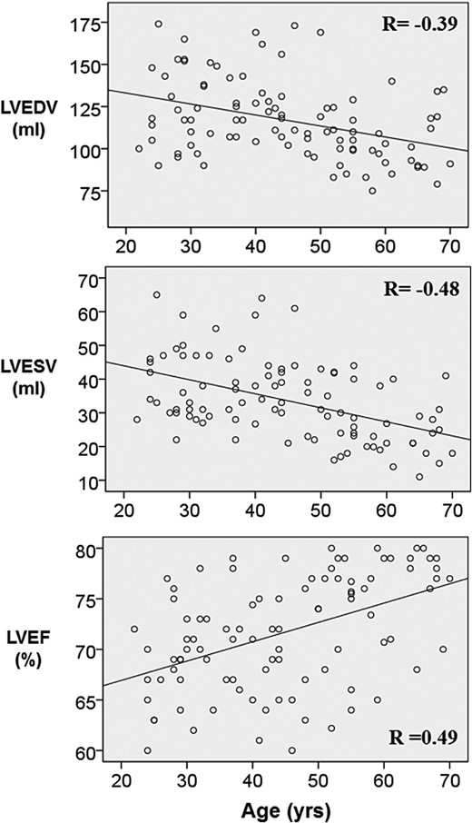
The relationship between age and myocardial volumes. Age was negatively correlated with LV volumes and positively correlated with LV ejection fraction. The correlation coefficient R is shown for each relationship (P < 0.001 for all).
Feasibility
Out of 1600 short-axis and 600 long-axis segments (total 2200) potentially available for the study population, 1600 segments (100%) were adequately tracked. Based on one investigator, semi-automatic border delineation took 5.6 ± 1.2 min.
Strain
Peak systolic strains and strain rates are shown in Table 2. Peak systolic Ell was −21.0 ± 4.1% at the endocardium and −17.3 ± 4.1% at the epicardium. Peak systolic Ecc was −26.5 ± 3.8% and −10.8 ± 2.5% at the endocardium and epicardium, respectively. Peak systolic Err was the highest, with a transmural value of 39.8 ± 8.3%. All peak systolic strains were higher at the endocardium than at the epicardium; this transmural strain gradient was greatest in the circumferential direction.
Peak systolic strain and systolic and diastolic strain rates
| Peak systolic strain (%) | Peak systolic SR (s−1) | Early diastolic SR (s−1) | |
|---|---|---|---|
| Longitudinal | |||
| Endocardial | −21.3 ± 4.8 | −1.22 ± 0.36 | 1.25 ± 0.39 |
| −11.9 to −30.7 | −0.51 to −1.93 | 0.49 to 2.01 | |
| Epicardial | −17.3 ± 4.1 | −0.99 ± 0.30 | 0.97 ± 0.33 |
| −9.3 to −25.3 | −0.40 to −1.58 | 0.32 to 1.62 | |
| Mean | −19.1 ± 4.1 | −1.11 ± 0.30 | 1.11 ± 0.33 |
| −11.1 to −27.1 | −0.52 to −1.70 | 0.46 to 1.76 | |
| Circumferential | |||
| Endocardial | −26.1 ± 3.8 | −1.56 ± 0.29 | 1.43 ± 0.35 |
| −18.7 to −33.5 | −0.99 to −2.13 | 0.74 to 2.12 | |
| Epicardial | −10.8 ± 2.5 | −0.61 ± 0.13 | 0.53 ± 0.18 |
| −5.9 to −15.7 | −0.36 to −0.86 | 0.18 to 0.88 | |
| Mean | −18.4 ± 2.9 | −1.09 ± 0.19 | 0.99 ± 0.24 |
| −12.7 to −24.1 | −0.72 to −1.46 | 0.52 to 1.46 | |
| Radial | |||
| Endocardial | 39.8 ± 8.3 | 1.63 ± 0.36 | −1.54 ± 0.48 |
| 23.5 to 56.1 | 0.92 to 2.34 | −0.60 to 2.48 | |
Results presented as mean ± SD and 95% confidence intervals.
The peak systolic Ecc was lower in the mid cavity than at the base or apex (P < 0.001 for both). Peak systolic Ecc measured in the mid cavity correlated strongly with that measured at the base (r = 0.71) and apex (r = 0.60) (P < 0.001 for both). As shown in Table 3, segmental peak systolic Ecc was heterogeneous.
Regional circumferential straina
| Peak systolic circumferential strain (%) | ||||
|---|---|---|---|---|
| Apical | Mid | Basal | P (all levels) | |
| Global | −29.3 ± 6.2 | −26.1 ± 3.8 | −28.4 ± 4.2 | P < 0.001 |
| Anterior | −25.6 ± 7.9 | −28.6 ± 6.8 | −27.6 ± 8.0 | P = 0.002 |
| Anteroseptal | −30.6 ± 8.2 | −24.7 ± 6.1 | −28.8 ± 8.6 | P < 0.001 |
| Septal | −24.6 ± 6.0 | −32.3 ± 8.1 | P < 0.001 | |
| Inferior | −32.1 ± 7.9 | −29.0 ± 6.3 | −31.7 ± 8.5 | P = 0.001 |
| Inferolateral | −26.0 ± 6.6 | −28.5 ± 9.3 | P = 0.006 | |
| Lateral | −28.8 ± 7.0 | −25.8 ± 7.1 | −26.2 ± 9.1 | P = 0.003 |
| P (all segments) | P < 0.001 | P < 0.001 | P < 0.001 | |
aValues presented as mean ± SD.
P-values refer to comparison of segments and slices by repeated-measures ANOVA.
Associations of strain and strain rate
Peak systolic Ecc (−25.6 vs. −26.5%, P = 0.23) and peak systolic Err (−38.8 vs. −40.9%, P = 0.20) were similar among males and females. There were significant gender differences (P < 0.001) in peak systolic Ell, with greater deformation in females (−22.7%) than in males (−19.3%).
There was a linear increase in the magnitude of peak systolic Ecc with advancing age (P = 0.01, β = 0.07); however, the increase in Ecc was greatest for those subjects over the age of 50 years. Accordingly, polynomial regression (with a quadratic curve) had superior modelling power [R2 = 0.11 (vs. 0.06 for linear), P = 0.003] (Figure 4). Table 4 shows age-adjusted values for peak systolic Ecc at the endocardium derived using the best-fit regression model. There was no such relationship when peak systolic Ecc was measured epicardially. There was no association between age and peak systolic Ell or Err. Similarly, there was no association between age and peak systolic SRcc or peak early diastolic SRcc (Table 5).
Age-adjusted mean endocardial peak systolic Ecc
| Age | Ecc |
|---|---|
| 20 | 26.7 |
| 30 | 25.6 |
| 40 | 25.4 |
| 50 | 26.3 |
| 60 | 28.1 |
| 70 | 31.0 |
| Age | Ecc |
|---|---|
| 20 | 26.7 |
| 30 | 25.6 |
| 40 | 25.4 |
| 50 | 26.3 |
| 60 | 28.1 |
| 70 | 31.0 |
Age-adjusted peak systolic Ecc calculated using the regression formula, Ecc = 0.005x2– 0.363x + 31.94, where x = age.
Regression analyses of circumferential strain and strain rate measures
| Independent variables | Peak systolic Ecc | Peak systolic SRcc | Peak early diastolic SRcc | ||||||
|---|---|---|---|---|---|---|---|---|---|
| R | Beta coefficient (95% CI) | P | R | Beta coefficient (95% CI) | P | R | Beta coefficient (95% CI) | P | |
| Univariable analyses | |||||||||
| Age (years) | 0.25 | 0.07 (0.2 to 0.12) | 0.01 | 0.10 | 0.00 (−0.01 to 0.01) | 0.89 | 0.10 | 0.00 (−0.01 to 0.00) | 0.32 |
| Sex (M = 1, F = 2) | 0.12 | 0.90 (−0.60 to 2.40) | 0.24 | 0.07 | 0.04 (−0.08 to 0.16) | 0.49 | 0.13 | 0.09 (−0.05 to 0.23) | 0.21 |
| Height (m) | −0.14 | −0.05 (−0.13 to 0.03) | 0.19 | 0.04 | 0.00 (−0.01 to 0.01) | 0.73 | −0.12 | 0.00 (−0.01 to 0.00) | 0.26 |
| Weight (kg) | −0.16 | −0.05 (−0.11 to 0.01) | 0.13 | 0.00 | 0.00 (−0.01 to 0.01) | 0.99 | −0.21 | −0.01 (−0.01 to 0) | 0.26 |
| BSA (kg/m2) | −0.16 | −3.2 (−7.3 to 0.90) | 0.13 | 0.00 | 0.03 (−0.31 to 0.31) | 0.98 | −0.20 | −0.38 (−0.76 to −0.01) | 0.05 |
| Heart rate (bpm) | 0.06 | 0.02 (−0.11 to 0.03) | 0.21 | 0.27 | −0.01 (−0.01 to 0.00) | 0.01 | 0.23 | 0.01 (0.00 to 0.02) | 0.02 |
| SBP (mmHg) | 0.21 | 0.07 (0.00 to 0.13) | 0.04 | 0.11 | 0.00 (0.00 to 0.01) | 0.29 | 0.06 | 0.00 (0.00 to 0.01) | 0.61 |
| DBP (mmHg) | −0.06 | 0.03 (−0.14 to 0.08) | 0.57 | −0.17 | −0.01 (−0.02 to 0.00) | 0.10 | −0.15 | −0.01 (−0.02 to 0.00) | 0.15 |
| LVEDV (mL) | −0.23 | −0.04 (−0.07 to −0.01) | 0.02 | −0.19 | −0.01 (−0.01 to 0.00) | 0.07 | 0.23 | 0.01 (0.00 to 0.01) | 0.02 |
| LVEDV (mL/m2) | −0.18 | −0.07 (−0.14 to 0.01) | 0.08 | −0.23 | −0.01 (−0.01 to 0.00) | 0.10 | −0.09 | 0.00 (−0.01 to 0.01) | 0.41 |
| LVEF (%) | 0.63 | 0.39 (0.29 to 0.49) | <0.001 | 0.47 | 0.02 (0.01 to 0.03) | <0.001 | 0.38 | 0.02 (0.01 to 0.03) | <0.001 |
| Multivariable analyses | |||||||||
| Age (years) | 0.02 | 0.00 (−0.07 to 0.08) | 0.90 | – | – | – | – | – | – |
| BSA (kg/m2) | – | – | – | – | – | – | −0.12 | −0.19 (−0.55 to 0.18) | 0.32 |
| Heart rate (bpm) | – | – | – | 0.19 | −0.01 (−0.01 to 0.00) | 0.07 | −0.15 | 0.00 (−0.01to 0.00) | 0.15 |
| SBP (mmHg) | 0.26 | 0.08 (0.01 to 0.15) | 0.02 | – | – | – | – | – | – |
| DBP (mmHg) | – | – | – | 0.14 | 0.01 (0.00 to 0.01) | 0.18 | – | – | – |
| LVEDV (mL) | −0.30 | −0.50 (−0.87 to −0.01) | 0.01 | 0.17 | 0.00 (0.00 to 0.01) | 0.11 | 0.22 | 0.00 (0.00 to 0.01) | 0.07 |
Ecc and SRcc have been analysed as positive numbers to aid interpretation of relationships.
Variables that reached a P-value of <0.10 were included in multivariable models (with exception of LVEF given its correlation with strain measures).
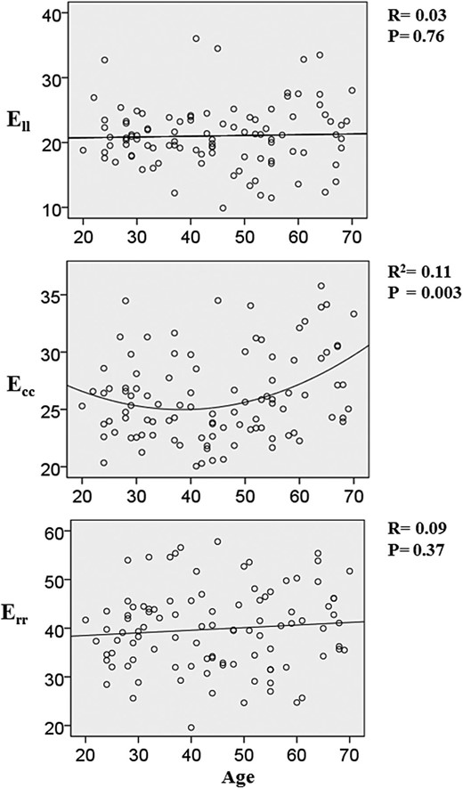
The relationship between age and myocardial strain. These scatter diagrams show the relationship between age and peak systolic longitudinal strain (Ell), peak systolic circumferential strain (Ecc), and peak systolic radial strain (Err). The best-fit linear regression line and correlation coefficient R are shown for the relationship between age and Ell and Err. The relationship between age and Ecc is shown as a quadratic curve as this had significantly superior modelling power.
As shown in Table 5, systolic BP (P = 0.04), LVEDV (P = 0.02), and LVEF (P < 0.001) also emerged as predictors of peak systolic Ecc on linear regression analyses. The relationship between systolic BP and peak systolic Ecc is also shown in Figure 5. In multivariable analysis, SBP (P = 0.02) and LVEDV (P = 0.01) remained significant predictors. With respect to peak systolic SRcc, heart rate (P = 0.01) and LVEF (P < 0.001) emerged as predictors. For peak early diastolic SRcc, body surface area (P = 0.03), heart rate (P = 0.006), LVEDV (P = 0.02), and LVEF (P < 0.001) emerged as predictors.
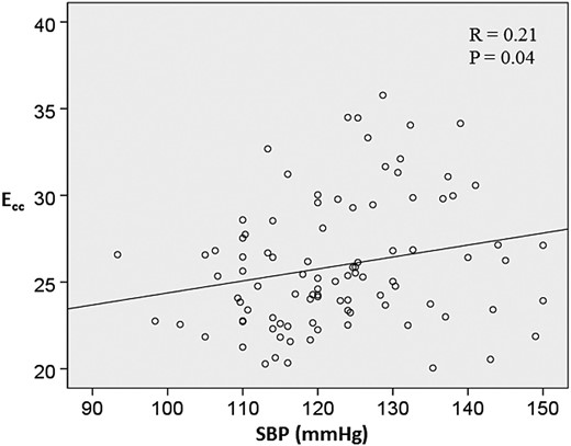
The relationship between systolic blood pressure and circumferential strain. This scatter diagram shows the relationship between systolic blood pressure (SBP) and circumferential strain (Ecc). The best-fit linear regression line and correlation coefficient R are also shown.
In a Supplementary data online, Table S1, we have shown that gender (P < 0.001), height (P = 0.001), weight (P = 0.009), body surface area (P < 0.001), SBP (P = 0.09), and LVEDV (P = 0.03) were all predictors of peak systolic Ell on linear regression analyses. BSA (P = 0.08) then gender (P = 0.12) had the greatest influence on Ell in multivariable analyses.
Reproducibility
Table 6 shows both intra- and inter-observer variability. In Bland–Altman analyses, peak systolic Ecc had the best intra- (bias, −0.34 ± 0.87; 95% CI, −2.05 to 1.36) and inter- (bias, 0.63 ± 1.29; 95% CI, −1.90 to 3.16) observer agreement. Of the three axial strains, peak systolic Err had the largest intra- (−0.03 ± 3.65; 95% CI, −7.2 to 7.1) and inter- (0.13 ± 6.4; 95% CI, −12.44 to 12.71) observer biases. All parameters had an intra-observer ICC of ≥0.85. All circumferential and longitudinal parameters had an inter-observer ICC of ≥0.85, but this coefficient was lower for radial parameters.
Intra-observer and inter-observer variability
| Variable | Variability | Mean bias ± SD | Limits of agreement | P | Coefficient of variation (%) | ICC (95% CI) |
|---|---|---|---|---|---|---|
| Peak systolic Err | Intra-observer | −0.03 ± 3.65 | −7.19 to 7.14 | 0.97 | 8.90 | 0.85 (0.66 to 0.94) |
| Inter-observer | 0.13 ± 6.41 | −12.44 to 12.71 | 0.93 | 14.67 | 0.55 (0.11 to 0.81) | |
| Peak systolic Ecc | Intra-observer | −0.34 ± 0.87 | −2.05 to 1.36 | 0.09 | 3.55 | 0.96 (0.90 to 0.99) |
| Inter-observer | 0.63 ± 1.29 | −1.90 to 3.16 | 0.06 | 4.95 | 0.93 (0.81 to 0.97) | |
| Peak systolic Ell | Intra-observer | −0.49 ± 1.83 | −4.08 to 3.11 | 0.29 | 7.68 | 0.88 (0.72 to 0.96) |
| Inter-observer | 0.22 ± 1.13 | −1.99 to 2.42 | 0.42 | 5.48 | 0.98 (0.94 to 0.99) | |
| Peak systolic SRrr | Intra-observer | −0.01 ± 0.14 | −0.29 to 0.27 | 0.74 | 8.68 | 0.89 (0.74 to 0.95) |
| Inter-observer | −0.03 ± 0.27 | −0.56 to 0.49 | 0.61 | 15.01 | 0.71 (0.38 to 0.88) | |
| Peak systolic SRcc | Intra-observer | −0.02 ± 0.08 | −0.18 to 0.13 | 0.21 | 5.36 | 0.96 (0.90 to 0.98) |
| Inter-observer | 0.02 ± 0.11 | −0.20 to 0.23 | 0.56 | 6.68 | 0.94 (0.84 to 0.98) | |
| Peak systolic SRll | Intra-observer | 0.02 ± 0.18 | −0.34 to 0.38 | 0.70 | 17.89 | 0.89 (0.72 to 0.96) |
| Inter-observer | 0.02 ± 0.16 | −0.30 to 0.33 | 0.61 | 12.95 | 0.86 (0.67 to 0.95) | |
| Peak early diastolic SRrr | Intra-observer | 0.03 ± 0.18 | −0.33 to 0.38 | 0.52 | 11.67 | 0.88 (0.72 to 0.95) |
| Inter-observer | −0.04 ± 0.48 | −0.98 to 0.90 | 0.72 | 26.77 | 0.50 (0.05 to 0.78) | |
| Peak early diastolic SRcc | Intra-observer | 0.00 ± 0.07 | −0.13 to 0.13 | 0.92 | 5.29 | 0.97 (0.93 to 0.99) |
| Inter-observer | −0.01 ± 0.11 | −0.24 to 0.21 | 0.63 | 7.82 | 0.96 (0.89 to 0.98) | |
| Peak early diastolic SRll | Intra-observer | 0.05 ± 0.18 | −0.30 to 0.40 | 0.27 | 14.84 | 0.85 (0.64 to 0.94) |
| Inter-observer | 0.01 ± 0.28 | −0.53 to 0.55 | 0.90 | 20.99 | 0.85 (0.63 to 0.94) |
Discussion
In this study, we have provided normal reference values for LV myocardial strain using FT-CMR, derived from a well-characterized group of healthy individuals with tailored age and sex stratification. All circumferential and longitudinal based variables had excellent intra- and inter-observer variability, and although agreement was less for radial parameters, these still had acceptable reproducibility. Our definition of a normal range for strain and strain rate measures using FT-CMR has emerged in the context of a promising role for this technique to detect preclinical disease, as shown by stress CMR studies.19,20 Further studies are undoubtedly needed to determine the role of FT-CMR in both clinical and research environments. At this stage, however, an accepted definition of normal values is paramount.
Normal values
There are key differences between the FT-CMR motion analysis techniques presented herein and those reported using other methodologies. In this respect, FT-CMR measures myocardial strain at both the endocardial and epicardial border, while speckle tracking measures strain from a region of interest within the myocardium. The presence of a transmural myocardial strain gradient is likely to confound comparisons of strain measures derived from speckle-tracking echocardiography and FT-CMR. Furthermore, there are differences between vendors of speckle-tracking echocardiography with regard to the regions at which strain is calculated. Some manufacturers derive strain from the mid-myocardium, whereas others permit endocardial and epicardial strain computation. The recently published consensus statement aims to standardize strain calculation as at present comparison of values between software is problematic.21 To allow for such gradients, FT-CMR global peak strain was expressed as the mean strain of values derived from the endocardial and epicardial borders. Accordingly, global strain values are comparable to those reported from the largest single normal reference population (250 patients) studied with speckle-tracking echocardiography which determined mid-myocardial strains. Marwick et al.22 found a mean peak systolic Ell of −18.6% compared with −19.1% in our study. Mean peak systolic Ecc was also similar (−18.7 vs. −18.4%) and peak systolic SRll was also comparable (−1.10 vs. −1.11 s−1).
Since there is no agreed normal reference range for diastolic strain parameters, current consensus currently suggests restricting their use to research applications.21 Nevertheless, early diastolic strain rate is a sensitive early marker of diastolic dysfunction and provides important information about LV relaxation and interstitial fibrosis.23 Moreover, measures of diastolic function predict incident heart failure and, therefore, carry prognostic significance.24 Thus far, CMR-based assessment of diastolic function using myocardial tagging has been restricted by loss of tags. In contrast, FT-CMR offers a more robust method, because it is not adversely affected by T1 relaxation. Our derivation of a normal reference range for early diastolic strain rate is therefore a key aspect of this study as it may have future clinical relevance. However, the lower temporal resolution of CMR (25 Hz in this study) compared with echocardiography raises concerns over whether any CMR-based deformation algorithm is apt for the assessment of early diastolic filling (the fastest part of the cardiac cycle). However, due to the nature of FT-CMR (like speckle tracking), the algorithms are more accurate at detecting rapid movements (there is a lower limit of pixel velocity that can be tracked from one frame to the next). While increasing the frame rate beyond normal acquisition protocols would enhance the quantification of early diastolic strain rate in this population, this may actually reduce the accuracy of strain calculation because of the trade off in spatial resolution. Further studies to elucidate the optimal spatial and temporal resolution for global and segmental strain assessment in health and disease are required.
The large standard deviation of peak strains within the normal population is similar to that reported with other methodologies.25 In view of the small measurement bias for repeated measures (both inter- and intra-observer) in our cohort, and the reported good intra-subject reproducibility in global measures with repeated imaging,26 this large spread within this population is likely due to normal biological variation.
Effects of age and sex on strain
Our findings of greater longitudinal deformation in women (but similar circumferential deformation) corroborate with those of Augustine et al.27 who have recently reported on strain values in 116 healthy subjects. Their study comprised young healthy volunteers with a narrow age distribution (age 29 ± 7 years). Our study also shows that these gender variations persist across a broad age spectrum. Moreover, we also report an age-related change in circumferential strain, which is in keeping with a recent 3D speckle-tracking echocardiography study.28 Accordingly, an age-related increase in LV torsion has been recognized, although the biomechanical reasons for this are still debated.29 Our multivariable regression analyses suggest that age-related changes in LVEDV and SBP (even within a normotensive population) are important factors in this respect. On the other hand, we have not shown any age-dependent variations in longitudinal strain. This is in contrast with Kuznetsova et al.30 who reported a decrease in the magnitude of longitudinal strain, associated with ageing, measured using tissue Doppler imaging in a mixed population of healthy individuals and hypertensive patients. Dalen et al.31 also reported an inverse relationship between age and longitudinal strain measured using tissue Doppler imaging in a large population of healthy individuals. Importantly, however, myocardial strain measured using tissue Doppler imaging is not necessarily comparable to speckle-tracking imaging. Notwithstanding, our findings of an absence of age-dependent variations in longitudinal myocardial strain is in keeping with the aforementioned speckle-tracking imaging study.22
Reproducibility and feasibility
In the present study, the best reproducibility was obtained for peak systolic Ecc, followed by peak systolic Ell and then peak systolic Err. Acceptable intra- and inter-observer agreement was also found for strain rate, in particular for peak systolic and peak early diastolic SRcc. This is consistent with the findings of Morton et al.26 who found that circumferential strain had the best inter-study variability on three serial CMR acquisitions over 1 day. Conversely, radial strain had the lowest reproducibility. This may relate to the fact that, as opposed to circumferential strain, radial strain is derived from both endocardial and epicardial motion and, therefore, its quantification relies on the simultaneous tracking of two regions of interest. In this respect, the contrast in signal intensity at the epicardial border is less prominent than that at the endocardial border. This is a likely cause for the comparatively low reproducibility of radial strain.
Reproducibility does not necessarily equate to accuracy. Theoretically any myocardial deformation algorithm could repeatedly quantify strain with a similar but inaccurate result. The robust reproducibility of this myocardial deformation algorithm may be a result of its highly automated process and background smoothing utilized. However, agreement with myocardial tagging is reassuring. Peak systolic Ecc can be measured with good agreement and peak systolic Ell with satisfactory agreement compared with the ‘gold standard’ myocardial tagging techniques.10,11 Validation of any radial parameters is more challenging as this is generally less accurately quantified by all deformation algorithms. The ‘acid test’ for this modality will be whether it can be used to assess preclinical disease, and these normal values will be useful in this respect.
As we have learnt from myocardial tagging, proving feasibility is a necessary step in the development of a clinically applicable imaging modality. In this study, we were able to track 100% of available segments. This is a potential advantage of FT-CMR over echocardiography, insofar as the latter is limited by foreshortening at the apex and ‘drop-out’ of the apical and anterolateral segments on the apical views. In addition, the sector widths required to image dilated hearts during echocardiography often result in frame rates that are suboptimal for speckle tracking.
Clinical and research applications
FT-CMR tracks the motion of anatomical structures over time. Tissue inhomogeneities and their variance in signal are important. While prominent differences in signal intensity between the myocardial and blood interface mean this methodology is well suited to measuring global strains, motion components parallel to tissue boundaries are more vulnerable to noise than perpendicular motion, and agreement for regional measures is therefore more modest.32,33 Thus, with its rapidity to execute and the lack of requirement of specialized acquisitions, FT-CMR lends itself to clinical use more readily than myocardial tagging. An ideal example is the serial assessment of patients undergoing cytotoxic chemotherapy.34 New guidelines for cardio-oncology mandate the reporting of global longitudinal strain,35 and FT-CMR may be appropriate for patients in whom poor acoustic windows prevent repeated speckle-tracking echocardiography. However, when the assessment of regional function is required, such as for the assessment of regional ischaemia, the differentiation of adjacent regions of myocardium provided by myocardial tags gives this clear advantages over FT-CMR.
Likewise, speckle-tracking echocardiography tracks acoustic interference patterns that are within the myocardium so is better suited to the regional assessment of function than FT-CMR. Neither CMR-based methodology can rival the much wider availability or speed of acquisition of echocardiographic-based measures. The disadvantages of speckle tracking have already been highlighted.
One attraction of FT-CMR is that cine images do not need any prior manipulation at acquisition as do myocardial tagging required to facilitate techniques using HARP or SPAMM analysis. In addition to saving time, this permits the retrospective study of cohorts. However, such historical data may have suboptimal frame rates for use with the FT-CMR algorithm. Caution is required if such cohorts are compared with the normal values presented herein.
Limitations
Our 100% yield relates to the high quality of our SSFP cines, and we acknowledge that the same image quality will not always be obtainable in a clinical environment, not least because arrhythmias may interfere with ECG gating. However, the diagnostic yield reported here compares favourably to that achieved by Marwick et al.22 who only obtained diagnostic quality images in 79% of healthy enrollees while compiling normal values for speckle-tracking. We present mean segmental values for circumferential but not longitudinal strain as sagittal LV outflow tract cines were not part of our acquisition protocol. Our finding that Ecc was lower in the mid cavity than at the base is in contrast to tagging studies.36 Although we cannot be assured of the reason for this discrepancy, it is plausible that, despite our slice selection protocol that was designed to negate the influence of through plane distortion from the LV outflow tract, this was an issue.
Conclusions
We have defined normal values for strain for healthy individuals using FT-CMR. Undoubtedly, this technique will undergo refinements in the future, as data from different disease groups and applications emerge. As with any imaging modality, normal values may vary according to software manufacturer and particular algorithms. It is imperative, therefore, that values quoted herein are expressed in the context of the technology used in the present study.
Authors' contributions
Project conception and design was by F.L. and R.J.T. Patient enrolment was conducted by W.E.M. Strain analysis was conducted by R.J.T. and W.E.M. with expert supervision from F.L. and R.S. Statistical analysis was performed by R.J.T. The first draft of the manuscript was written by R.J.T. with all authors revising the piece critically before agreeing on the final manuscript. F.L. supervised the project.
Acknowledgements
The authors are grateful to Peter Nightingale for his advice on statistical methods, and Medtronic, Inc. and St Jude Medical for providing financial support for this project. W.E.M. is supported by a British Heart Foundation Clinical Research Fellowship Grant. We are also indebted to the Wellcome/NIHR Clinical Research Facility and the University of Birmingham for providing resources that have allowed us to conduct this research.
References
Author notes
These authors contributed equally to this work.
